Other articles in the cycle
. I
. II
. II
The formal theory of modeling uses algebraic relations, including them in the signatures of models of algebraic structures, which describe real physical, technical objects and the processes of their functioning. This publication is a continuation of the previous one , the reading of which is desirable, since many concepts and terms used here are described there.
The presentation is offered not in the traditional (arrow) style, but in the way that I myself had to imagine and master this whole kitchen both from textbooks / manuals and from magazine articles. I consider the catalog that I have created to be especially useful, it allows you to select almost any space and present its elements in a convenient form: a matrix, a graph, etc. You can immediately see what you are dealing with and properties (they have already been written out) often do not need to be checked.
Relationship concept
I think that the term attitude is familiar to every reader, but asking for a definition will confuse most. There are many reasons for this. They are most often in teachers who, if they used relationships in the teaching process, did not focus on this term, did not give memorable examples. Some commentators on the article attributed the comments to their own account and added minuses. But you can't hide a sewing in a sack. There were no serious publications, and no. Ask yourself, have you worked with any relationship space? And honestly answer yourself. What can you tell the world about this space? To begin with, at least list its elements and specify properties. You even look at the DBMS through the eyes of their creators, but they don't see everything either, or they don't show everything, as, for example, in microcircuits.
I'll do a little repetition here. One should start with the abstract set A = {a1, a2, a3, ..., an}. You can read about it here . For better understanding, we will reduce the set to 3 elements, i.e. A = {a1, a2, a3}. Now we carry out the Cartesian multiplication × = 2 and explicitly enumerate all the elements of the Cartesian square
× = {(a1, a1), (a1, a2), (a1, a3), (a2, a1), (a2, a2 ), (a2, a3), (a3, a1), (a3, a2), (a3, a3)}.
We got 9 ordered pairs of elements from A × A, in a pair the first element is from the first factor, the second from the second. Now let's try to get all subsets from the A × A Cartesian square. The subsets will contain a different number of pairs: one, two, three, and so on up to all 9 pairs, we also include the empty set ∅ in this list. How many subsets are there? Many, namely 2 9= 512 elements.
Definition . A subset of a Cartesian square set is called a binary relation. If the Cartesian square of two factors, the ratio is binary, if of 3 it is internal, of 4 it is tetrar, and of n it is n-ary. Arity is the number of places in a relationship element.
Definition . The set of all subsets of the set A is called a Boolean. Boolean consists of 2 | A | elements, here | A | Is the cardinality of the set.
Relationships can be defined in different ways:
- enumeration of elements; R1 = {(a2, a2), (a2, a3), (a3, a1)}; R2 = {(a3, a3)}
- binary vector; <000011100>; <000000001>
- matrix;
- graph and other ways.
Next, we move on to considering spaces of relations, assuming that the concept, properties of relations and operations with them are familiar to the reader at least to the extent of our publication in the link.
Binary relation spaces
Let's preliminarily clarify that relationships can be strict (these are all anti-reflective relationships) or non-strict (all others). We will focus on the relationship of indifference and preference, the latter are subdivided into weak preferences and strict preferences (for some reason, not strong). In general, there is no order in science with terminology and most likely there will not be. In cryptography, for example, removing a cipher from a cryptogram in the presence of a key is decryption, and without a key, decryption. It would seem that a decoder decodes, but no.
The space of binary relations with a carrier set is an arbitrary subset of the set of binary relations given on. Consider the main spaces for preference relationships (Figure 2.15).
R- the space of all relations of weak preference, satisfy the condition of reflexivity and completeness.
QT - weak preferences satisfying the quasi-transitivity condition.
QO is the space of linear quasi- orders , that is, relations from QT that are transitive.
TO is the space of all perfect orders, that is, relations from QO that are antisymmetric.
SP is the space of all relations of strict preference; they satisfy the properties of antireflexivity and antisymmetry.
RO- relations of strict partial order, or transitive strict preferences. Since the relations of strict partial order are transitive, it is natural to use them to represent them by reduced graphs, that is, those in which the arcs realizing transitivity are omitted. Such abbreviated graphs are called Hasse diagrams.
QS is the space of quasiseries, that is, strict partial orders for which the relation I = ¬ (PUP -1 ) is an equivalence.
TSO is the space of strict linear orders, that is, those partial orders for which the completeness property is satisfied.
It should be noted that there are n of such relations in total! .. For example, for n = 3, the number of perfect relations is 6, and they are all shown in Fig. 2.13.
T- the space of all relations of tolerance (indifference), they have the properties of symmetry and reflexivity.
TOT is the space of transitively oriented tolerance relations, that is, relations such that the complement to I is represented as a union of mutually inverse transitive relations, i.e.,
¬I = R∩R -1 .
I is the space of all equivalence relations, that is, symmetric, reflexive and transitive relations.
E - space of relations of equality, consists of one relation represented by a diagonal matrix. There is a one-to-one relationship between the spaces R, P and I, determined by the mapping of preference relations.


Figure 2.15 Scheme of spaces of binary relations
The revealed connections between the spaces are used to transfer decision-making problems (DM) from one space to another, where they can be solved in a simpler way, and then the resulting solution is returned to the original space, where the DP was formulated.
These relationships are shown diagrammatically in Fig. 2.14. Spaces of binary relations (types of relations) are shown in Fig. 2.15.
Equivalence relations
Definition . A binary relation σ ⊆ A × A, which has three properties of reflexivity, symmetry, transitivity, is called a binary equivalence relation (BOE). The equivalence relation σ (x, y), (x, y) ∊σ, xσy, x≈y is denoted. It is convenient to use a matrix (tabular) representation of the relationship. Below in Figure 2.24 is just a matrix representation. Above the set of 4 elements, there are 15 BOEs, which are all depicted.
Representation and analysis of the structure of equivalence relations (n = 4)
Equivalence from binary relations is perhaps the most common BO. Rarely does science manage without this concept, but even when equivalences are used to state any questions, it can be difficult to understand what the author meant. Even with the correct definition and enumeration of the properties inherent in this binary relation, the difficulties of perception remain.
Let's start with an example on equivalences, which illustrates the limitations of their number.
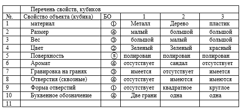
Example 1 . Let there be three cubes. Let's make a list of the properties that the cubes are endowed with and the practical use of which (the properties of the cubes) makes them seem interchangeable. Let us assign numbers to the cubes, and represent their properties in Table 1.
For each of the properties, BOE and equivalence classes arise. Continuing the list of properties, we will not get new equivalence relations. There will only be repetitions of the already built ones, but for other signs. Let us show the connection between BOE and sets.
Consider a set of three elements A = {1,2,3} and obtain for it all possible partitions into all parts. ①1 | 2 | 3; ②12 | 3; ③13 | 2; ④ 1 | 23; ⑤123. The last split into one part. Partition numbers and BOs in circles.
Definition . A partition of a set A is a family i, i = 1 (1) I, of nonempty pairwise disjoint subsets from , the union of which forms the entire original set = Ui, i∩j = ∅, ∀ i ≠ j. The sub-sets i are called equivalence classes of the partition of the original set.
These are all partitions of the set (5 pieces). The BO analysis shows that there are also only 5 different equivalence relations. Is this coincidence a coincidence? We can associate each partition with a matrix of nine cells (3 × 3 = 9), each of which either contains an ordered pair of elements from set A, or the cell remains empty if there is no object for the corresponding pair. The rows and columns of the matrix are marked with elements of the set A, and the row-column intersection corresponds to an ordered pair (i, j). It is not a pair that fits into the matrix cell, but simply one or zero, however, zero is often not written at all.
No, the coincidence is not accidental. It turns out that each partition of the set is in one-to-one correspondence with the BOE, and the cardinality of the set can be any | A | = n.
This relationship is perhaps the most frequent in terms of use in scientific circulation, but the set of properties realized in this regard greatly limits its prevalence.
So among all abstract binary relations over a set of three elements (there are 2 9 = 512 relations in total ), only five are equivalences - carriers of the required properties, less than one percent.
For | A | = 4 relations exist 2 16= 65536, but there are only 15 equivalences. This is a very rare type of relationship. On the other hand, equivalence relations are widespread in applied problems. Wherever there are and are considered sets of very different objects and different partitions of such sets (not numbers) into parts, equivalence relations arise. They can be called mathematical (algebraic) models of such partitions, which classify sets of objects according to various criteria.
The minimal partition of the set A formed from one-element subsets A = U {a} and the partition A consisting of the set {A} itself are called trivial (improper) partitions.
Lattice P (4): all partitions of the set A = {a1, a2, a3, a4} = {1,2,3,4}

The minimum partitioning corresponds to the equivalence relation P15, which is called equality or a unit relation. Each equivalence class contains a single element. To a partition of the set A, which includes only the set A itself, there corresponds an equivalence relation containing all the elements of the Cartesian square A × A.

The closest type to equivalence relations is tolerance relations . The set of tolerance relations contains all equivalence relations. For carrier A there are three elements of tolerance 8. All of them have the properties of reflexivity and symmetry.
When the transitivity property is fulfilled, five of the eight tolerances transforms into equivalences (Figures 2.24 and 2.25).
Definition . The set of equivalence classes [a] σ of the elements of the set A is called the quotient set (denoted by A / σ) of the set A by the equivalence σ.
Definition . A natural (canonical) mapping f: A → A / σ is a mapping f such that f (a) = [a] σ.
Tolerance relations and their analysis
These BOs have already been mentioned earlier, but here we will consider them in more detail. Everyone knows the concepts of similarity, similarity, similarity, indistinguishability, interchangeability of objects. They seem to be similar in content, but not the same thing. When only similarity is indicated for objects, it is impossible to break them down into clear classes so that within a class the objects are similar, and there is no similarity between objects of different classes. In the case of similarity, a vague situation arises without clear boundaries. On the other hand, the accumulation of insignificant differences in similar objects can lead to completely dissimilar objects.
In the previous part, we discussed the meaningful meaning of the relation of similarity (equivalence) of objects. Equally important is the situation when it is necessary to establish the similarity of objects.
Let the shape of geometric bodies be studied. If the similarity of the shape of objects, for example, cubes, means their complete interchangeability in a certain learning situation, then the similarity is partial interchangeability (when among the cubes there are parallelepipeds very similar to them), that is, the possibility of interchangeability with some (admissible in this situation ) losses.
The greatest measure for similarity is indistinguishability, not at all the sameness, as it might seem at first glance. Identity is a qualitatively different property. Identity can only be viewed as a special case of indistinguishability and similarity.
The point is that indistinguishable objects (as well as similar, similar ones) cannot be divided into classes so that the elements in each class do not differ, and the elements of different classes are obviously different.
Indeed, we will consider the set of points (x, y) on the plane. Let the value d have a value less than the eye's resolvability threshold, that is, d is such a distance at which two points located at this distance merge into one, i.e. visually indistinguishable (at the chosen distance of the plane from the observer). Consider now n points lying on one straight line and spaced (each from neighboring) at a distance d. Each pair of
adjacent points is indistinguishable, but if n is large enough, the first and last points will be far apart from each other and will certainly be distinguishable.
The traditional approach to studying similarity or indistinguishability is to first determine the measure of similarity, and then examine the relative position of similar objects. The English mathematician Zieman, studying models of the visual apparatus, proposed an axiomatic definition of similarity. Thus, it became possible to study the properties of similarity regardless of how exactly it is specified in a given situation: the distance between objects, the coincidence of some features, or the subjective opinion of the observer.
Let us introduce an explication of the concept of similarity or indistinguishability.
Definition . The relation T on the set M is called the relation of tolerance or tolerance if it is reflexive and symmetric.
The correctness of this definition is evident from the fact that the object is obviously indistinguishable from itself and, of course, looks like itself (this gives the reflexivity of the relationship). The order of consideration of two objects does not affect the final conclusion about their similarity or dissimilarity (symmetry).
From the example with visual indistinguishability of points on the plane, we see that the transitivity of tolerance is not fulfilled for all pairs of objects.
It is also clear that since similarity is a special case of similarity, then equivalence must be a special case of tolerance. Comparing the definitions of equivalence and tolerance, we are convinced that this is the case. The philosophical principle: "the particular is richer than the general" is clearly confirmed. An additional property - transitivity makes some of the tolerance relations equivalences. Two twins are so much alike that they can take exams for each other without risk. However, if two students are only alike, then such a trick, although feasible, is risky.
Each element of the set carries certain information about elements similar to it. But not all the information, as in the case of identical elements. Here, different degrees of information are possible that one element contains in relation to another.
Let's consider examples where tolerance is set in different ways.
Example 2 . The set M consists of four-letter Russian words - common nouns in the nominative case. We will call such words similar if they differ by no more than one letter. The well-known problem "Turning a fly into an elephant" in precise terms is formulated as follows. Find a sequence of words beginning with the word "fly" and ending with the word "elephant", any two adjacent words in which are similar in the sense of the definition just given. The solution to this problem:
fly - mura - tura - tara - kara - kare - cafe - kaffr - musher - skiff - hook - croc - time - stock - groan - elephant.
Example 3... Let p be a natural number. We denote by Sp the collection of all non-empty subsets of the set M = {1, 2, ..., p}. The relation “have at least one common element” on the set Sp is a tolerance relation. Then two such subsets are called tolerant if they have at least one common element. It is easy to see that the reflexivity and symmetry of the relationship is fulfilled.
The set Sp is called a (p –1) -dimensional simplex. This concept generalizes the concept of a segment, triangle and tetrahedron to the multidimensional case. The numbers 1, 2, 3, ..., p are interpreted as vertices of a simplex. Two-element subsets - as edges, three-element - as flat (two-dimensional) faces, other k-element subsets - as (k –1) -dimensional faces. The number of all elements (subsets) of Sp is equal to 2 p - 1.
Tolerance of subsets (faces) means that they have common vertices.
Definition . The set M with the tolerance relation τ given on it is called the space of tolerance. Thus, the space of tolerance is a pair (M, τ).
Example 4 . The space of tolerance Sp can be generalized to the infinite case. Let H be an arbitrary set. If SH is the collection of all non-empty subsets of the set H, then the tolerance relation T on SH is given by the condition: X T Y if X∩Y ≠ ∅. The symmetry and reflexivity of this relationship is obvious. The SH space is designated <H, T> and is called the "universal" space of tolerance.
Example 5... Let p be a natural number. We denote by Bp the set of all points of the p-dimensional space whose coordinates are equal to 0 or 1. Tolerance in Bp is given by the rule: xτy if x and y contain at least one coinciding component (coordinate). The total number of elements in Bp is 2 r . For each element x = (a1, a2, ..., ap) from the set Bp, there is only one element y = (1 − a1, 1 − a2, ..., 1 − ap) that is not tolerant to it.
Obviously, Bp consists of all vertices of the p-dimensional cube.
Example 6 . Consider the space of tolerance, the components of which take on any real values.
In particular, this is the set of all points x = (a1, a2) in the Cartesian plane. Tolerance of two points means that they have at least one coordinate. This means that two tolerant points are either on a common vertical or on a common horizontal.
For other values of p, the space can be interpreted as a set of points in p-dimensional space. In particular, each element x can be considered a numerical function defined on the set of natural numbers {1, 2, 3, ...}, which assigns to each natural number i: 1 ≤ i ≤ p a real number ai (a finite number sequence). Then the tolerance of two functions x and y means that they are equal at least at one point.
Partial order relations and their analysis
Ordered sets are sets with an order relation introduced on it. Definition . A set A and a binary order relation R on it (≤) is called partially ordered if the relation holds (as in BOE) three conditions (one condition is different):
- reflexivity ∀ x ∊ A (xRx); (antireflexivity ∀ x ∊ A ¬ (xRx));
- antisymmetry ∀ , y ∊ (Ry yRx → x = y);
- transitivity ∀ x, y, z ∊ A (xRy & yRz → xRz).
With an anti-reflective attitude, a strict partial order arises . The set B (A) of all subsets of the set A, ordered by the inclusion of elements, is a partially ordered set (PN). The partially ordered set (B (A), ⊆) is often called a Boolean.
An element x∊A POZA A covers an element y∊A if x> y and there is no z∊A such that x> z> y. A pair of elements x, y∊A is called comparable if x ≥ y or x ≤ y.
If in PLA A every pair of its elements is comparable, then A is called a linearly ordered set or chain .
If some plague B consists only of elements incomparable with each other, then the set B is called an antichain... A chain in PLAG A is called saturated if it cannot be nested in any other chain other than itself.
The saturated antichain is defined similarly. A maximum chain (antichain) is a chain (antichain) containing the maximum number of elements.
An element m of a PLM A is called minimal if there is no element ∊ in other than m and such that ≤m. An element M of a plague A is called maximal if there is no element x “greater” than M, other than M and such that x ≥ M.
An element y∊A of a plague A is called maximal if ∀ x∊ A x ≤ y. The element y∊ A PLAG A is called the smallestif ∀ x∊A x ≥ y. For the largest and smallest elements, it is customary to use the designations 1 and 0, respectively. They are called universal boundaries. Any plague A has at most one smallest and at most one largest element. In PLA A, several minimum and several maximum elements are permissible.It is
convenient to depict the final PLA A with a Hasse diagram , which is a directed graph, its vertices are distributed over the levels of the diagram and correspond to elements from A, and each arc is directed downwards and is drawn if and only if the element x∊A covers the element y∊A.
Transitive arcs are not drawn. Hasse chart levels contain elements of the same rank, i.e. connected with the minimum elements of the PCM by paths of equal length (by the number of arcs).
Let B be a non-empty subset of PLA A, then an element x∊A is called the exact upper bound (denoted by sup A B) of the set B if x ≥ y for all y∊B and if it follows from the truth of the relation z ≥ y for all y∊B, that z ≥ x.
The exact lower bound (denoted by inf A B) of a set B is an element x∊A if x ≤ y for all y∊B and if the condition z ≤ y for all y∊ B implies that z ≤ x.
Example 7 . Two finite numerical sets
A = {0,1,2, ..., 21} and B = {6,7,10,11} are given.
CHUM (A, ≤) is shown in Fig. 2.26.
The collection B Δ of all upper bounds for is called the upper cone for the set B. The collection ∇of all the lower faces for B is called the lower cone for B.

Any subset of PLA is also PLP with respect to inherited order. If the set contains the largest and / or smallest elements, then they are maximum (minimum, respectively). The converse is not true. Boolean has a single smallest (Ø) and a single largest element.
In the given set, the smallest element is zero (0) and it coincides with the only minimal element, and the largest element does not exist. The maximum elements are {19, 20, 21}. The exact upper bound for B = {6,7,10,11} is element 21 (this is the smallest element in the upper cone).
General situation. Let a set be given, the cardinality of which is *******. Of all the binary relations that are possible on this set, let us single out the binary preference relations and the related strict partial order relations.
Partial orders differ from strict partial orders only in that they contain additional elements (in the matrix representation - diagonal) (i, ai) = 1, i = 1 (1) n, and the number of those and other orders in the complete set of relations the same. Until now, no dependencies (formula, algorithm) have been found that would allow one to calculate and enumerate the number of partial orders for any n.
Different authors have determined and published the following results by direct calculation (Table 2.12).
The computational experiments of the author made it possible to obtain not only the number, but also the form (representation) of partial orders at different powers of the multiplier-carrier of relations. The printer choked on printing such huge lists, but not only beauty requires sacrifices, science also does not refuse them.

Table 2.12 shows: n = | A | - the cardinality of the set-carrier; the second line is the number of all binary relations on the set A; and further
| In (n) | - the number of classes of non-isomorphic relations;
| (n) | - the number of relations of partial order;
| Gn (n) | - the number of classes of non-isomorphic partial order relations;
| Gl (n) | = n! - the number of linear order relations.
As you can see, in the table for small n, for example, G (n = 4), there are only 219, data are given, the values of which grow very rapidly with increasing n, which significantly complicates their quantitative (and qualitative) direct analysis, even with a computer.
The table below illustrates the possibility of generating Γ (n = 4) of all partial orders from the intersection of each with each linear partial order. But in this situation, redundant (repetitive) ones arise, which for small n can be cut off manually (recalculated). It turns out 300 matrices, but there are only 219 PLs among them. General formulas have not been obtained. At the global level, the situation is similar, although I have not seen any publications about PLM transfers by Western authors. Our algorithms are completely original and pioneering.
I will give a possible scheme for solving the problem of enumerating the elements of the space of partial orders (n = 4).

The set of strict partial orders in the lexicographic ordering of linear orders (n = 4) is generated by their mutual intersection.


Several important definitions of mathematics, for concepts that are often found in texts.
Definition . A closed interval is a set of the form {x: a ≤ x ≤ b}; an open interval is not closed, and a half-open interval, that is, a set of the form {x: a <x ≤ b}, where a <b, or of the form {x: a ≤ x <b} is neither open nor closed.
Definition . The boundary of an arbitrary interval of a real line in the usual topology of real numbers consists only of the ends of this interval, regardless of whether this interval is open, closed, or half-open. The boundary of the set of rational numbers, as well as the boundary of the set of all irrational numbers, is the entire set of real numbers.
Definition... Every linearly ordered set, in any non-empty subset of which there is the smallest element, is called well-ordered.
Definition . A family R is called a chain (sometimes a tower, a nest) if and only if, for any of its elements A and B, either A ⊂ B or B ⊂ A. This condition is equivalent to the assertion that the family R is linearly ordered by inclusion or, in the accepted terminology - that the family R together with the inclusion relation is a chain.
P r and n c and p m a to s and m al n about s t and H a u s d o r f a. For any family of sets A and any nest R formed by elements of the family A, there is a maximal nest M in A containing R.
An important theorem on sets and their families (J.L. Kelly "General topology" p. 55).
Theorem. (a) PRINTSIpMakSIMALN about ELEMENT. A maximal element in the family A of a set exists if, for each nest in A, there is an element in A that contains an arbitrary element of this nest.
(b) PRINTSIpMINIMALNO ELEMENT. The smallest element in a family A exists if, for each nest in A, there is an element in A that is contained in each element of this nest.
(c) Lemma T yuk and. Each family of sets of finite character has a maximal element.
(d) LEMMA KURATOVSKOGO. Every chain in a (partially) ordered set is contained in some maximal chain.
(e) Tson's lemma. If each chain of some partially ordered set is bounded from above, then this set has a maximal element.
(f) A to s and o m and a choice. Let Xα be a non-empty set for every element a from the set of indices A. Then there exists a function c on A such that c (a) ∊ Xα for each a from A.
(g) Postulate Tserm elo. For any family A of disjoint nonempty sets, there is a set C such that AUC for each A from A consists of exactly one point.
(h) PRINTS and P in full order of delivery. Each set can be completely ordered.