Linear Regression Basics

Hello, Habr!



The purpose of this article is to talk about linear regression, namely, to collect and show the formulations and interpretations of the regression problem in terms of mathematical analysis, statistics, linear algebra and probability theory. Although the textbooks set out this topic strictly and exhaustively, another popular science article will not hurt.



! Watch out for traffic! The article contains a noticeable number of images for illustrations, some in gif format.

Content

• Introduction
• Least square method
  • Mathematical analysis
  • Statistics
  • Probability theory
• Multilinear regression
  • Linear algebra
• Arbitrary basis
• Concluding remarks
  • Dimension selection problem
  • Numerical methods
• Advertising and conclusion

Introduction

There are three similar concepts, three sisters: interpolation, approximation and regression.

They have a common goal: from a family of functions, choose the one that has a certain property.





Interpolation- a way to select from a family of functions the one that passes through the given points. The function is then usually used to calculate at intermediate points. For example, we manually set the color to several points and want the colors of the remaining points to form smooth transitions between the given ones. Or we set keyframes for the animation and want smooth transitions between them. Classic examples: Lagrange polynomial interpolation, spline interpolation, multidimensional interpolation (bilinear, trilinear, nearest neighbor, etc.). There is also a related concept of extrapolation - predicting the behavior of a function outside of an interval. For example, predicting the dollar rate based on previous fluctuations is extrapolation.



Approximation- a way to choose from a family of "simple" functions an approximation for a "complex" function on a segment, while the error should not exceed a certain limit. Approximation is used when you need to get a function similar to a given one, but more convenient for calculations and manipulations (differentiation, integration, etc.). When optimizing critical sections of the code, an approximation is often used: if the value of a function is calculated many times per second and absolute accuracy is not needed, then a simpler approximant with a lower "cost" of calculation can be dispensed with. Classic examples include Taylor series on a segment, orthogonal polynomial approximation, Padé approximation, Bhaskar sine approximation, etc.



Regression- a way to choose from a family of functions the one that minimizes the loss function. The latter characterizes how much the trial function deviates from the values ​​at the given points. If points are obtained in an experiment, they inevitably contain measurement error, noise, so it is more reasonable to require that the function convey the general trend, and not exactly pass through all the points. In a sense, regression is an “interpolating fit”: we want to draw the curve as close to the points as possible and still keep it as simple as possible to capture the overall trend. The loss function (in the English literature “loss function” or “cost function”) is responsible for the balance between these conflicting desires.



In this article, we'll look at linear regression. This means that the family of functions from which we choose is a linear combination of predetermined basis functions$$${f_i}$

$$

$$f = \sum_i w_i f_i.$$

The goal of regression is to find the coefficients of this linear combination, and thereby determine the regression function $$$f$ (also called amodel). I note that linear regression is called linear precisely because of the linear combination of basis functions - this is not related to the most basic functions (they can be linear or not).



Regression has been with us for a long time: the method was first published by Legendre in 1805, although Gauss came to it earlier and used it successfully to predict the orbit of the "comet" (actually a dwarf planet) Ceres. There are many variations and generalizations of linear regression: LAD, Least Squares, Ridge Regression, Lasso Regression, ElasticNet, and many others.

Least square method

Let's start with the simplest two-dimensional case. Let us be given points on the plane$$$\{(x_1,y_1),\cdots,(x_N,y_N)\}$ and we are looking for such an affine function

$$

$$f(x) = a + b \cdot x,$$

so that its graph is closest to the points. Thus, our basis consists of a constant function and a linear$$$(1, x)$ .



As you can see from the illustration, the distance from a point to a straight line can be understood in different ways, for example, geometrically - it is the length of a perpendicular. However, in the context of our task, we need a functional distance, not a geometric one. We are interested in the difference between experimental value and model prediction for each$$$x_i,$ so you need to measure along the axis$$$y$ .



The first thing that comes to mind is to try an expression that depends on the absolute values ​​of the differences as a loss function$$$|f(x_i) - y_i|$... The simplest option is the sum of the deviation modules$$$\sum_i |f(x_i) - y_i|$ results in Least Absolute Distance (LAD) regression.



However, the more popular loss function is the sum of the squares of the deviations of the regressant from the model. In English literature, it is called Sum of Squared Errors (SSE)

$$

$$\text{SSE}(a,b)=\text{SS}_{res[iduals]}=\sum_{i=1}^N{\text{}_i}^2=\sum_{i=1}^N(y_i-f(x_i))^2=\sum_{i=1}^N(y_i-a-b\cdot x_i)^2,$$

Least Squares (OLS) - Linear Regression with $$$\text{SSE}(a,b)$ as a loss function.



This choice is primarily convenient: the derivative of a quadratic function is a linear function, and linear equations are easily solved. However, further I will indicate other considerations in favor of$$$\text{SSE}(a,b)$ .

Mathematical analysis

The simplest way to find $$$\text{argmin}_{a,b} \, \text{SSE}(a,b)$ - calculate partial derivatives with respect to$$$a$ and$$$b$ , equate them to zero and solve the system of linear equations

$$

$$\begin{aligned} \frac{\partial}{\partial a}\text{SSE}(a,b)&=-2\sum_{i=1}^N(y_i-a-bx_i), \\ \frac{\partial}{\partial b}\text{SSE}(a,b)&=-2\sum_{i=1}^N(y_i-a-bx_i)x_i. \end{aligned}$$

The values ​​of the parameters that minimize the loss function satisfy the equations

$$

$$\begin{aligned} 0 &= -2\sum_{i=1}^N(y_i-\hat{a}-\hat{b}x_i), \\ 0 &= -2\sum_{i=1}^N(y_i-\hat{a}-\hat{b}x_i)x_i, \end{aligned}$$

which are easy to solve

$$

$$\begin{aligned} \hat{a}&=\frac{\sum_i y_i}{N}-\hat{b}\frac{\sum_i x_i}{N},\\ \hat{b}&=\frac{\frac{\sum_i x_i y_i}{N}-\frac{\sum_i x_i\sum_i y_i}{N^2}}{\frac{\sum_i x_i^2}{N}-\left(\frac{\sum_i x_i^2}{N}\right)^2}. \end{aligned}$$

We got unwieldy and unstructured expressions. Now we will ennoble them and breathe meaning into them.

Statistics

The resulting formulas can be compactly written using statistical estimators: mean $$$\langle{\cdot}\rangle$ , variations$$$\sigma_{\cdot}$ (standard deviation), covariance$$$\sigma({\cdot},{\cdot})$ and correlations$$$\rho({\cdot},{\cdot})$

$$

$$\begin{aligned} \hat{a}&=\langle{y}\rangle-\hat{b}\langle{x}\rangle, \\ \hat{b}&=\frac{\langle{xy}\rangle-\langle{x}\rangle\langle{y}\rangle}{\langle{x^2}\rangle-\langle{x}\rangle^2}. \end{aligned}$$

Let's rewrite $$$\hat{b}$ as

$$

$$\hat{b} = \frac{\sigma(x,y)}{\sigma_x^2},$$

Where $$$\sigma_x$ is the uncorrected (biased) standard sample deviation, and $$$\sigma(x,y)$- covariance. Now, remember that the correlation coefficient (Pearson's correlation coefficient)

$$

$$\rho(x,y)=\frac{\sigma(x,y)}{\sigma_x \sigma_y}$$

and write

$$

$$\hat{b}=\rho(x,y)\frac{\sigma_y}{\sigma_x}.$$

Now we can appreciate all the elegance of descriptive statistics by writing the regression line equation like this

$$

$$\boxed{y-\langle {y} \rangle = \rho(x,y)\frac{\sigma_y}{\sigma_x}(x-\langle {x} \rangle)}.$$

First, this equation immediately indicates two properties of the regression line:

• the straight line passes through the center of mass $$$(\langle{x}\rangle, \langle{y}\rangle)$;
• if along the axis $$$x$ per unit of length choose $$$\sigma_x$, and along the axis $$$y$ - $$$\sigma_y$, then the slope of the straight line will be from $$$-45^\circ$ before $$$45^\circ$... This is due to the fact that$$$-1 \leq\rho(x,y)\leq 1$...

Secondly, now it becomes clear why the regression method is called that way. In units of standard deviation$$$y$ deviates from its mean by less than $$$x$, because $$$|\rho(x,y)|\leq1$... This is called regression (from the Latin regressus - "return") in relation to the mean. This phenomenon was described by Sir Francis Galton in the late 19th century in his article "Regression to Mediocrity in the Inheritance of Growth." The article shows that traits (such as height) that deviate greatly from the mean are rarely inherited. The characteristics of the offspring seem to tend to the average - nature rests on the children of geniuses.



By squaring the correlation coefficient, we obtain the coefficient of determination$$$R = \rho^2$... The square of this statistical measure shows how well the regression model fits the data.$$$R^2$equal to $$$1$, means that the function fits perfectly to all points - the data is perfectly correlated. It can be proved that$$$R^2$shows how much of the variance in the data is due to the best linear model. To understand what this means, we introduce the definitions

$$

$$\begin{aligned} \text{Var}_{data} &= \frac{1}{N}\sum_i (y_i-\langle y \rangle)^2, \\ \text{Var}_{res} &= \frac{1}{N} \sum_i (y_i-\text{}(x_i))^2, \\ \text{Var}_{reg} &= \frac{1}{N} \sum_i (\text{}(x_i)-\langle y \rangle)^2. \end{aligned}$$

$$$\text{Var}_{data}$ - variation of initial data (variation of points $$$y_i$).



$$$\text{Var}_{res}$ - variation of residuals, that is, variation of deviations from the regression model - from $$$y_i$ you need to subtract the model's prediction and find the variation.



$$$\text{Var}_{reg}$ - variation of regression, i.e. variation of the predictions of the regression model at points $$$x_i$ (note that the mean of the model predictions is the same as $$$\langle y \rangle$).



The fact is that the variation in the original data is decomposed into the sum of two other variations: the variation that is explained by the model, and variation of the random noise (residuals)

$$

$$\boxed{{\color{red}{\text{Var}_{data}}} ={\color{green}{\text{Var}_{res}}}+ {\color{blue}{\text{Var}_{reg}}}.}$$

or

$$

$$\sigma^2_{data} =\sigma^2_{res}+ \sigma^2_{reg}.$$

As you can see, the standard deviations form a right-angled triangle.





We strive to get rid of the variability associated with noise and leave only the variability that is explained by the model - we want to separate the wheat from the chaff. The extent to which the best of the linear models succeeded is evidenced by$$$R^2$equal to one minus the fraction of error variation in the total variation

$$

$$R^2=\frac{\text{Var}_{data}-\text{Var}_{res}}{\text{Var}_{data}}=1-\frac{\color{green}{\text{Var}_{res}}}{\color{red}{\text{Var}_{data}}}$$

or the proportion of variation explained (proportion of regression variation in total variation)

$$

$$R^2=\frac{\color{blue}{\text{Var}_{reg}}}{\color{red}{\text{Var}_{data}}}.$$

$$$R$ equal to the cosine of an angle in a right triangle $$$(\sigma_{data}, \sigma_{reg}, \sigma_{res})$... By the way, sometimes a fraction of the unexplained variation is introduced $$$FUV=1-R^2$and it is equal to the square of the sine in this triangle. If the coefficient of determination is small, perhaps we chose unsuccessful basis functions, linear regression is not applicable at all, etc.

Probability theory

Earlier we came to the loss function $$$\text{SSE}(a,b)$for reasons of convenience, but it can also be reached using the theory of probability and the method of maximum likelihood (MLM). Let me briefly recall its essence. Suppose we have$$$N$independent identically distributed random variables (in our case, measurement results). We know the form of the distribution function (for example, the normal distribution), but we want to determine the parameters that are included in it (for example$$$\mu$ and $$$\sigma$). To do this, you need to calculate the probability of getting$$$N$datapoints under the assumption of constant, yet unknown parameters. Due to the independence of the measurements, we get the product of the probabilities of each measurement. If we think of the resulting value as a function of parameters (likelihood function) and find its maximum, we get an estimate of the parameters. Often, instead of the likelihood function, they use its logarithm - it is easier to differentiate it, but the result is the same.



Let's go back to the simple regression problem. Let's say that the values$$$x$ we know exactly, but in measurement $$$y$there is random noise ( weak exogenous property ). Moreover, we assume that all deviations from the straight line ( linearity property ) are caused by noise with a constant distribution ( constant distribution ). Then

$$

$$y = a + bx + \epsilon,$$

Where $$$\epsilon$ - normally distributed random variable

$$

$$\epsilon \sim \mathcal{N}(0,\,\sigma^{2}), \qquad p(\epsilon) = \frac{1}{\sqrt{2 \pi \sigma^2}} e^{-\frac{\epsilon^2}{2\sigma^2}}.$$

Based on the assumptions above, we write down the likelihood function

$$

$$\begin{aligned} L(a,b|\mathbf{y})&=P(\mathbf{y}|a,b)=\prod_i P(y_i|a,b)=\prod_i p(y_i-a-bx|a,b)=\\ &= \prod_i \frac{1}{\sqrt{2 \pi \sigma^2}} e^{-\frac{(y_i-a-bx)^2}{2\sigma^2}}= \frac{1}{\sqrt{2 \pi \sigma^2}}e^{-\frac{\sum_i (y_i-a-bx)^2}{2 \sigma^2}}=\\ &= \frac{1}{\sqrt{2 \pi \sigma^2}}e^{-\frac{\text{SSE}(a,b)}{2 \sigma^2}} \end{aligned}$$

and its logarithm

$$

$$l(a,b|\mathbf{y})=\log{L(a,b|\mathbf{y})}=-\text{SSE}(a,b)+const.$$

Thus, the maximum likelihood is achieved at a minimum $$$\text{SSE}$

$$

$$(\hat{a},\hat{b})=\text{argmax}_{a,b} \, l(a,b|\mathbf{y}) = \text{argmin}_{a,b} \, \text{SSE}(a,b),$$

which gives reason to accept it as a loss function. By the way, if

$$

$$\begin{aligned} \epsilon \sim \text{Laplace}(0, \alpha), \qquad p_{L}(\epsilon; \mu, \alpha) =\frac{\alpha}{2}e^{-\alpha |\epsilon-\mu|} \end{aligned}$$

we get the LAD regression loss function

$$

$$E_{LAD}(a,b)=\sum_i |y_i-a-bx_i|,$$

which we mentioned earlier.



The approach we have used in this section is one possible one. It is possible to achieve the same result using more general properties. In particular, the property of constancy of distribution can be weakened by replacing it with the properties of independence, constancy of variation (homoscedasticity) and absence of multicollinearity. Also, instead of MMP estimation, you can use other methods, for example, linear MMSE estimation.

Multilinear regression

So far, we have considered the regression problem for one scalar feature $$$x$, however usually the regressor is $$$n$-dimensional vector $$$\mathbf{x}$... In other words, for each dimension, we register$$$n$features, combining them into a vector. In this case, it is logical to accept the model with$$$n+1$ independent basis functions of the vector argument - $$$n$ degrees of freedom correspond $$$n$ features and one more - regressant $$$y$... The simplest choice is linear basis functions$$$(1, x_1, \cdots, x_n)$... When$$$n = 1$ we get the already familiar basis $$$(1, x)$...



So, we want to find such a vector (set of coefficients)$$$\mathbf{w}$, what

$$

$$\sum_{j=0}^n w_j x_j^{(i)}= \mathbf{w}^{\top}\mathbf{x}^{(i)} \simeq y_i, \qquad \qquad \qquad \qquad i=1\dots N.$$

Sign "$$$\simeq$"means that we are looking for a solution that minimizes the sum of the squared errors

$$

$$\hat{\mathbf{w}}=\text{argmin}_\mathbf{w} \, \sum_{i=1}^N \left({y_i - \mathbf{w}^{\top}\mathbf{x}^{(i)}}\right)^2$$

The last equation can be rewritten in a more convenient way. For this we place$$$\mathbf{x}^{(i)}$ in matrix rows (information matrix)

$$

$$X= \begin{pmatrix} - & \mathbf{x}^{(1)\top} & - \\ \cdots & \cdots & \cdots\\ - & \mathbf{x}^{(N)\top} & - \end{pmatrix} = \begin{pmatrix} | & | & & | \\ \mathbf{x}_0 & \mathbf{x}_1 & \cdots & \mathbf{x}_n \\ | & | & & | \end{pmatrix} = \begin{pmatrix} 1 & x^{(1)}_{1} & \cdots & x^{(1)}_{n} \\ \cdots & \cdots & \cdots & \cdots\\ 1 & x^{(N)}_{1} & \cdots & x^{(N)}_{n} \end{pmatrix}.$$

Then the columns of the matrix $$$\mathbf{x}_{i}$ meet measurements $$$i$-th feature. It is important not to get confused here:$$$N$ - the number of measurements, $$$n$- the number of signs (features) that we register. The system can be written as

$$

$$X \, \mathbf{w} \simeq \mathbf{y}.$$

The square of the norm of the difference between the vectors on the right and left sides of the equation forms the loss function

$$

$$\text{SSE}(\mathbf{w}) = {\|\mathbf{y}-X \mathbf{w}\|}^2, \qquad \qquad \mathbf{w} \in \mathbb{R}^{n+1}; \, \mathbf{y} \in \mathbb{R}^{N},$$

which we intend to minimize

$$

$$\begin{aligned} \hat{\mathbf{w}}&=\text{argmin}_\mathbf{w} \, \text{SSE}(\mathbf{w}) = \text{argmin}_\mathbf{w} \, (\mathbf{y}-X \mathbf{w})^{\top}(\mathbf{y}-X \mathbf{w})=\\ &= \text{argmin}_\mathbf{w} \,(\mathbf{y}^{\top}\mathbf{y}-2\mathbf{w}^{\top}X^{\top}\mathbf{y}+\mathbf{w}^{\top}X^{\top}X\mathbf{w}). \end{aligned}$$

Let's differentiate the final expression by $$$\mathbf{w}$(if you forgot how to do it, take a look at the Matrix cookbook )

$$

$$\frac{\partial \, \text{SSE}(\mathbf{w})}{\partial \mathbf{w}}=-2 X^{\top}\mathbf{y}+2 X^{\top}X\mathbf{w},$$

we equate the derivative to $$$\mathbf{0}$and we get the so-called. normal equations

$$

$$X^{\top}X \, \hat{\mathbf{w}}=X^{\top}\mathbf{y}.$$

If the columns of the information matrix $$$X$ are linearly independent (there are no perfectly correlated features), then the matrix $$$X^{\top}X$has the opposite (the proof can be seen, for example, in the video of Khan's academy ). Then we can write

$$

$$\boxed{\hat{\mathbf{w}} = (X^{\top}X)^{-1}X^{\top}\mathbf{y}=X^{+}\mathbf{y}},$$

Where

$$

$$X^{+}=(X^{\top}X)^{-1}X^{\top}$$

pseudo-inverse to $$$X$... The concept of a pseudoinverse matrix was introduced in 1903 by Fredholm, and it played an important role in the works of Moore and Penrose.



Let me remind you what to turn$$$X^{\top}X$ and find $$$X^{+}$ only possible if the columns $$$X$are linearly independent. However, if the columns$$$X$ close to linear dependence, calculation $$$(X^{\top}X)^{-1}$is already becoming numerically unstable. The degree of linear dependence of features in$$$X$or, as they say, the multicollinearity of the matrix$$$X^{\top}X$, can be measured by the conditionality number - the ratio of the maximum eigenvalue to the minimum. The bigger it is, the closer$$$X^{\top}X$ to degenerate and unstable computation of the pseudoinverse.

Linear algebra

The solution to the problem of multilinear regression can be reached quite naturally with the help of linear algebra and geometry, because even the fact that the norm of the error vector appears in the loss function already hints that the problem has a geometric side. We have seen that an attempt to find a linear model describing the experimental points leads to the equation

$$

$$X \, \mathbf{w} \simeq \mathbf{y}.$$

If the number of variables is equal to the number of unknowns and the equations are linearly independent, then the system has a unique solution. However, if the number of dimensions exceeds the number of features, that is, there are more equations than unknowns, the system becomes inconsistent, overdetermined. In this case, the best we can do is choose the vector$$$\mathbf{w}$whose image $$$X\mathbf{w}$ the closest to $$$\mathbf{y}$... Let me remind you that many images or column space$$$\mathcal{C}(X)$ Is a linear combination of the column vectors of the matrix $$$X$

$$

$$\begin{pmatrix} | & | & & | \\ \mathbf{x}_0 & \mathbf{x}_1 & \cdots & \mathbf{x}_n \\ | & | & & | \end{pmatrix} \mathbf{w} = w_0 \mathbf{x}_0 + w_1 \mathbf{x}_1 + \cdots w_n \mathbf{x}_n .$$

$$$\mathcal{C}(X)$ - $$$n+1$-dimensional linear subspace (we consider features linearly independent), linear span of column vectors $$$X$... So if$$$\mathbf{y}$ belongs $$$\mathcal{C}(X)$, then we can find a solution, if not, we will seek, so to speak, the best of the unsolved.



If in addition to vectors$$$\mathcal{C}(X)$ we consider all vectors perpendicular to them, then we get one more subspace and we can any vector from $$$\mathbb{R}^{N}$decompose into two components, each of which lives in its own subspace. The second, perpendicular space can be characterized as follows (we will need this later). Let it go$$$\mathbf{v} \in \mathbb{R}^{N}$then

$$

$$X^\top \mathbf{v} = \begin{pmatrix} - & \mathbf{x}_0^{\top} & - \\ \cdots & \cdots & \cdots\\ - & \mathbf{x}_n^{\top} & - \end{pmatrix} \mathbf{v} = \begin{pmatrix} \mathbf{x}_0^{\top} \cdot \mathbf{v} \\ \cdots \\ \mathbf{x}_n^{\top} \cdot \mathbf{v} \\ \end{pmatrix}$$

is zero if and only if $$$\mathbf{v}$ perpendicular to all $$$\mathbf{x}_i$, and hence the whole $$$\mathcal{C}(X)$... Thus, we have found two perpendicular linear subspaces, linear combinations of vectors of which completely, without holes, "cover" all$$$\mathbb{R}^N$... This is sometimes denoted by the orthogonal direct sum symbol





Where $$$\text{ker}(X^{\top})=\{\mathbf{v}|X^{\top}\mathbf{v}=\mathbf{0}\}$... Each of the subspaces can be reached using the corresponding projection operator, but more on that below.



Now let's imagine $$$\mathbf{y}$ decomposition

$$

$$\mathbf{y} = \mathbf{y}_{\text{proj}} + \mathbf{y}_{\perp}, \qquad \mathbf{y}_{\text{proj}} \in \mathcal{C}(X), \qquad \mathbf{y}_{\perp} \in \text{ker}(X^{\top}).$$

If we are looking for a solution $$$\hat{\mathbf{w}}$, then it is natural to require that $$$|| \mathbf{y} - X\mathbf{w} ||$was minimal, because this is the length of the remainder vector. Taking into account the perpendicularity of subspaces and the Pythagorean theorem

$$

$$\text{argmin}_\mathbf{w} || \mathbf{y} - X\mathbf{w} || = \text{argmin}_\mathbf{w} || \mathbf{y}_{\perp} + \mathbf{y}_{\text{proj}} - X\mathbf{w} || = \text{argmin}_\mathbf{w} \sqrt{|| \mathbf{y}_{\perp} ||^2 + || \mathbf{y}_{\text{proj}} - X\mathbf{w} ||^2},$$

but since choosing a suitable $$$\mathbf{w}$, I can get any column space vector, then the problem is reduced to

$$

$$X\hat{\mathbf{w}} = \mathbf{y}_{\text{proj}},$$

and $$$\mathbf{y}_{\perp}$will remain as a fatal error. Any other choice$$$\hat{\mathbf{w}}$ will only make the mistake more.



If we now remember that $$$X^{\top} \mathbf{y}_{\perp} = \mathbf{0}$then it's easy to see

$$

$$X^\top X \mathbf{w} = X^{\top} \mathbf{y}_{\text{proj}} = X^{\top} \mathbf{y}_{\text{proj}} + X^{\top} \mathbf{y}_{\perp} = X^{\top} \mathbf{y},$$

which is very convenient, since $$$\mathbf{y}_{\text{proj}}$ we do not have, but $$$\mathbf{y}$- there is. Recall from the previous section that$$$X^{\top} X$ has the inverse under the condition of linear independence of features and write the solution

$$

$$\mathbf{w} = (X^\top X)^{-1} X^\top \mathbf{y} = X^{+} \mathbf{y},$$

Where $$$X^{+}$the already familiar pseudoinverse matrix. If we are interested in the projection$$$\mathbf{y}_{\text{proj}}$, then we can write

$$

$$\mathbf{y}_{\text{proj}} = X \mathbf{w} = X X^{+} \mathbf{y} = \text{Proj}_X \mathbf{y},$$

Where $$$\text{Proj}_X$- operator of projection onto column space.



Let's find out the geometric meaning of the coefficient of determination.



Note that the purple vector $$$\bar{y} \cdot \boldsymbol{1}=\bar{y} \cdot (1,1,\dots,1)^{\top}$ proportional to the first column of the information matrix $$$X$, which consists of one unit according to our choice of basis functions. In RGB triangle

$$

$${\color{red}{\mathbf{y}-\hat{y} \cdot \boldsymbol{1}}}={\color{green}{\mathbf{y}-\bar{\mathbf{y}}}}+{\color{blue}{\hat{\mathbf{y}}-\bar{y} \cdot \boldsymbol{1}}}.$$

Since this triangle is rectangular, then by the Pythagorean theorem

$$

$${\color{red}{\|\mathbf{y}-\hat{y} \cdot \boldsymbol{1}\|^2}}={\color{green}{\|\mathbf{y}-\bar{\mathbf{y}}\|^2}}+{\color{blue}{\|\hat{\mathbf{y}}-\bar{y} \cdot \boldsymbol{1}\|^2}}.$$

This is a geometric interpretation of the already known fact that

$$

$${\color{red}{\text{Var}_{data}}} = {\color{green}{\text{Var}_{res}}}+{\color{blue}{\text{Var}_{reg}}}.$$

We know that

$$

$$R^2=\frac{\color{blue}{\text{Var}_{reg}}}{\color{red}{\text{Var}_{data}}},$$

which means

$$

$$R=\cos{\theta}.$$

Nice, isn't it?

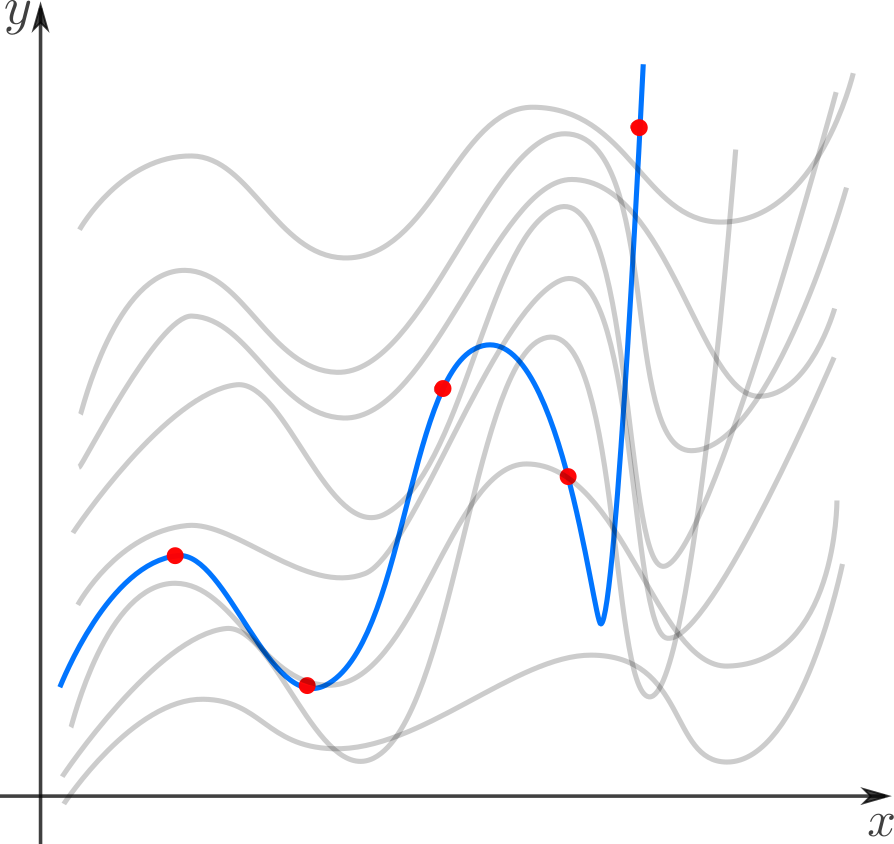
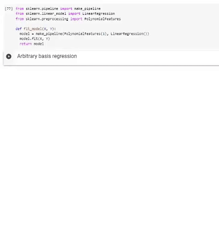
Arbitrary basis

As we know, regression is performed on basis functions $$$f_i$ and its result is the model

$$

$$f = \sum_i w_i f_i,$$

but so far we have used the simplest $$$f_i$that simply relayed the original features without changes, well, except that they supplemented them with constant features $$$f_0(\mathbf{x}) = 1$... As you can see, in fact, neither kind$$$f_i$, nor their number is limited by anything - the main thing is that the functions in the basis are linearly independent. Usually, the choice is made based on assumptions about the nature of the process that we are modeling. If we have reason to believe that the points$$$\{(x_1,y_1),\cdots,(x_N,y_N)\}$ fall on a parabola, and not on a straight line, then it is worth choosing a basis $$$(1, x, x^2)$... The number of basic functions can be either less or more than the number of original features.



If we have decided on the basis, then we proceed as follows. We form a matrix of information

$$

$$\Phi = \begin{pmatrix} - & \boldsymbol{f}^{(1)\top} & - \\ \cdots & \cdots & \cdots\\ - & \boldsymbol{f}^{(N)\top} & - \end{pmatrix} = \begin{pmatrix} {f}_{0}\left(\mathbf{x}^{(1)}\right) & {f}_{1}\left(\mathbf{x}^{(1)}\right) & \cdots & {f}_{n}\left(\mathbf{x}^{(1)}\right) \\ \cdots & \cdots & \cdots & \cdots\\ {f}_{0}\left(\mathbf{x}^{(N)}\right) & {f}_{1}\left(\mathbf{x}^{(N)}\right) & \cdots & {f}_{n}\left(\mathbf{x}^{(N)}\right) \end{pmatrix},$$

write the loss function

$$

$$E(\mathbf{w})={\|{\boldsymbol{\epsilon}}(\mathbf{w})\|}^2={\|\mathbf{y}-\Phi \, \mathbf{w}\|}^2$$

and find its minimum, for example, using the pseudoinverse matrix

$$

$$\hat{\mathbf{w}} = \text{argmin}_\mathbf{w} \,E(\mathbf{w}) = (\Phi^{\top}\Phi)^{-1}\Phi^{\top}\mathbf{y}=\Phi^{+}\mathbf{y}$$

or another method.

Concluding remarks

Dimension selection problem

In practice, it is often necessary to independently build a model of the phenomenon, that is, to determine how many and which basic functions should be taken. The first impulse to "get more" can play a cruel joke: the model will be too sensitive to noise in the data (overfitting). On the other hand, if you overly restrict the model, it will be too rough (underfitting).



There are two ways to get out of the situation. The first is to consistently increase the number of basic functions, check the quality of the regression and stop in time. Or the second: choose a loss function that will determine the number of degrees of freedom automatically. As a criterion for the success of the regression, you can use the coefficient of determination, which was already mentioned above, however, the problem is that$$$R^2$grows monotonically with increasing dimension of the basis. Therefore, the adjusted coefficient is introduced

$$

$$\bar{R}^2=1-(1-R^2)\left[\frac{N-1}{N-(n+1)}\right],$$

Where $$$N$ - sample size, $$$n$- the number of independent variables. Following the$$$\bar{R}^2$, we can stop in time and stop adding additional degrees of freedom.



The second group of approaches is regularization, the most famous of which is Ridge ($$$L_2$/ ridge / Tikhonov regularization), Lasso ($$$L_1$regularization) and Elastic Net (Ridge + Lasso). The main idea of ​​these methods is to modify the loss function with additional terms that will not allow the vector of coefficients$$$\mathbf{w}$ grow indefinitely and thus prevent retraining

$$

$$\begin{aligned} E_{\text{Ridge}}(\mathbf{w})&=\text{SSE}(\mathbf{w})+\alpha \sum_i |w_i|^2 = \text{SSE}(\mathbf{w})+\alpha \| \mathbf{w}\|_{L_2}^2,\\ E_{\text{Lasso}}(\mathbf{w})&=\text{SSE}(\mathbf{w})+\beta \sum_i |w_i| =\text{SSE}(\mathbf{w})+\beta \| \mathbf{w}\|_{L_1},\\ E_{\text{EN}}(\mathbf{w})&=\text{SSE}(\mathbf{w})+\alpha \| \mathbf{w}\|_{L_2}^2+\beta \| \mathbf{w}\|_{L_1}, \\ \end{aligned}$$

Where $$$\alpha$ and $$$\beta$- parameters that control the "strength" of the regularization. This is a vast topic with beautiful geometry that deserves a separate discussion. By the way, I will mention that for the case of two variables, using probabilistic interpretation, one can obtain the Ridge and Lasso regressions by successfully choosing the prior distribution for the coefficient$$$b$

$$

$$y = a + bx + \epsilon,\qquad \epsilon \sim \mathcal{N}(0,\,\sigma^{2}),\qquad \left\{\begin{aligned} &b \sim \mathcal{N}(0,\,\tau^{2})&\leftarrow\text{Ridge},\\ &b \sim \text{Laplace} (0,\,\alpha)&\leftarrow\text{Lasso}. \end{aligned}\right.$$

Numerical methods

Let me say a few words about how to minimize the loss function in practice. SSE is an ordinary quadratic function that is parameterized by the input data, so in principle it can be minimized by the steepest descent method or other optimization methods. Of course, the best results are shown by algorithms that take into account the form of the SSE function, for example, the stochastic gradient descent method. Lasso's implementation of regression in scikit-learn uses the coordinate descent method.



You can also solve normal equations using numerical linear algebra methods. An efficient method that scikit-learn uses for OLS is to find the pseudoinverse using singular value decomposition. The fields of this article are too narrow to touch on this topic, for details I advise you to refer to the course of lectures by K.V. Vorontsov.

Advertising and conclusion

This article is an abridged retelling of one of the chapters of a course on classical machine learning at the Kiev Academic University (successor to the Kiev branch of the Moscow Institute of Physics and Technology, KO MIPT). The author of the article helped create this course. The course is technically done on the Google Colab platform, which allows you to combine LaTeX formatted formulas, Python executable code, and interactive demonstrations in Python + JavaScript, so that students can work with the course materials and run the code from any computer that has a browser. The home page contains links to abstracts, practice workbooks, and additional resources. The course is based on the following principles:

• all materials must be available to students from the first pair;
• the lecture is needed for understanding, not for taking notes (notes are already ready, there is no point in writing them if you don't want to);
• a lecture is more than a lecture (there is more material in the notes than was announced at the lecture, in fact, the notes are a full-fledged textbook);
• visibility and interactivity (illustrations, photos, demos, gifs, code, videos from youtube).

If you want to see the result, take a look at the course page on GitHub .



I hope you were interested, thank you for your attention.