🤲🏽 ⁉️ 🙋🏿 Vector spaces 🌝 ❤️ 📹

When conducting scientific and applied research, models are often created in which points and / or vectors of certain spaces are considered. For example, elliptic curve cipher models use affine and projective spaces. They resort to projective ones when it is necessary to speed up calculations, since in the formulas for manipulating the points of an elliptic curve derived within the framework of the projective space, there is no operation of division by a coordinate, which cannot be circumvented in the case of an affine space .

The division operation is just one of the most "expensive" operations. The fact is that in algebraic fields, and accordingly in groups, there is no division operation at all, and the way out (when it is impossible not to divide) is that the division operation is replaced by multiplication, but multiplied not by the coordinate itself, but by its inverse value ... From this it follows that one must first involve the extended Euclidean GCD algorithm and something else. In short, not everything is as simple as portrayed by the authors of most publications about the ECC. Almost everything that has been published on this topic and not only on the Internet is familiar to me. Not only are the authors not competent and are engaged in profanity, the evaluators of these publications add authors in the comments, that is, they see neither gaps nor obvious errors. About a normal article, they write that it is already the 100500th and it has zero effect.So far everything is arranged on Habré, the analysis of publications is huge, but not the quality of the content. There is nothing to object here - advertising is the engine of business.

Linear vector space

The study and description of the phenomena of the surrounding world necessarily leads us to the introduction and use of a number of concepts such as points, numbers, spaces, straight lines, planes, coordinate systems, vectors, sets, etc.

Let r _<3>= <r1, r2, r3> vector of three-dimensional space, specifies the position of one particle (point) relative to the origin. If we consider N elements, then the description of their position requires specifying 3 ∙ N coordinates, which can be considered as the coordinates of some vector in 3N-dimensional space. If we consider continuous functions and their collections, then we come to spaces whose dimension is equal to infinity. In practice, they are often limited to using only the subspace of such an infinite-dimensional coordinate function space that has a finite number of dimensions.

Example 1 . Fourier series is an example of using function space. Consider the expansion of an arbitrary function in a Fourier series

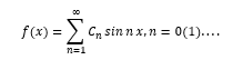
It can be interpreted as the expansion of the "vector" f (x) into an infinite set of "orthogonal" basis vectors sinnx

This is an example of abstraction and extension of the concept of a vector to an infinite number of dimensions. Indeed, it is known that for -π≤x≤π

The essence of further consideration will not suffer if we abstract from the dimension of the abstract vector space - be it 3, 3N or infinity, although for practical applications, finite-dimensional fields and vector spaces are of greater interest.

A set of vectors r1, r2,… will be called a linear vector space L if the sum of any two of its elements is also in this set and if the result of multiplying an element by a number C is also included in this set. Let's make a reservation right away that the values of the number C can be selected from a well-defined number set F - the field of residues modulo a prime number p, which is considered to be attached to L.

Example 2 . A set of 8 vectors made up of n = 5-bit binary numbers

r0 = 00000, r1 = 10101, r2 = 01111, r3 = 11010, r4 = 00101, r5 = 10110, r6 = 01001, r7 = 11100 forms the vector space L if the numbers C є {0,1}. This small example allows you to verify the manifestation of the properties of a vector space included in its definition.

The summation of these vectors is performed bitwise modulo two, that is, without transferring ones to the most significant bit. Note that if all C are real (in the general case C belong to the field of complex numbers), then the vector space is called real.

Formally, the axioms of the vector space are written as follows:

r1 + r2 = r2 + r1 = r3; r1, r2, r3 є L - addition commutativity and closedness;

(r1 + r2) + r3 = r1 + (r2 + r3) = r1 + r2 + r3 - addition associativity;

ri + r0 = r0 + ri = ri; ∀i, ri, r0 є L - existence of a neutral element;

ri + (- ri) = r0, for ∀i there is an opposite vector (-ri) є L;

1 ∙ ri = ri ∙ 1 = ri existence of a unit for multiplication;

α (β ∙ ri) = (α ∙ β) ∙ ri; α, β, 1, 0 are elements of the number field F, ri є L; multiplication by scalars is associative; the result of the multiplication belongs to L;

(α + β) ri = α ∙ ri + β ∙ ri; for ∀i, ri є L, α, β are scalars;

a (ri + rj) = ari + arj for all a, ri, rj є L;

a ∙ 0 = 0, 0 ∙ ri = 0; (-1) ∙ ri = - ri.

Dimension and basis of vector space

When studying vector spaces, it is of interest to clarify such questions as the number of vectors forming the entire space; what is the dimension of space; What is the smallest set of vectors, by applying to it the operation of summation and multiplication by a number, that makes it possible to form all the vectors of the space? These questions are fundamental and cannot be ignored, since without answers to them, the clarity of perception of everything else that makes up the theory of vector spaces is lost.

It turned out that the dimension of the space is closely related to the linear dependence of vectors, and to the number of linearly independent vectors that can be chosen in the space under study in many ways.

Linear independence of vectors

A set of vectors r1, r2, r3 ... r from L is called linearly independent if for them the relation

is satisfied only under the condition of simultaneous equality

с_{1} = с_{2} = \dots = с_{р} = 0

$_1=_2=…=_=0$ ...

All

с_{k}

$_k$ , k = 1 (1) p, belong to the number field of residues modulo two

F = {0, 1}.

If in some vector space L one can choose a set of p vectors for which the relation

c_{1} r_{1} + c_{2} r_{2} + . . . + c_{p} r_{p} = 0

$c_1 r_1+c_2 r_2+...+c_p r_p=0$ is executed, provided that not all

с_{k} = 0

$_k = 0$ simultaneously, i.e. in the field of deductions it turned out to be possible to select a set

с_{k}

$_k$ , k = 1 (1) , among which there are nonzero ones, then such vectors

r_{i}

$r_i$ are called linearly dependent.

Example 3 . Two vectors on the plane

е_{1}

$_1$ = <0, 1> ^T and

е_{2}

$_2$ = <1, 0> ^T are linearly independent, since in the relation (T-transposition)

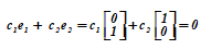
it is impossible to pick up any pair of numbers

с_{1}, с_{2}

$_1, _2$ coefficients not equal to zero at the same time for the ratio to be fulfilled.

Three vectors

е_{1}

$_1$ = <0, 1> ^T ,

е_{2}

$_2$ = <1, 0> ^T ,

е_{3}

$_3$ = <1, 1> ^T form a system of linearly dependent vectors, since in the relation

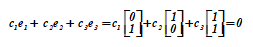
equality can be ensured by choosing the coefficients

с_{1} = с_{2} = 1, с_{3} = - 1

$_1 = _2 = 1, _3 = –1$ not equal to zero at the same time. Moreover, the vector

e_{3} = е_{1} + е_{2}

$e_3 = _1 + _2$ is a function

е_{1}

$_1$ and

е_{2}

$_2$ (their sum), which indicates the dependence

e_{3}

$e_3$ from

е_{1}

$_1$ and

е_{2}

$_2$ ... The proof of the general case is as follows.

Let at least one of the values

с_{k}

$_k$ , k = 1 (1) p, for example,

с_{р} \neq 0

$_ ≠ 0$ , and the relation is satisfied. This means that vectors

r_{k}

$r_k$ , k = 1 (1) , are linearly dependent

Let us explicitly separate the vector r

The vector r _p is said to be a linear combination of vectors

r_{1}, r_{2} \dots r_{р} - 1

$r_1, r_2… r_-1$ or r _p through the remaining vectors is expressed in a linear manner, i.e. r _p linearly depends on the others. He is their function.

On a two-dimensional plane, any three vectors are linearly dependent, but any two non-collinear vectors are independent. In 3D space, any three non-coplanar vectors are linearly independent, but any four vectors are always linearly dependent.

Dependence / independence of the population {

e_{1}, e_{2}, e_{3}, . . ., e_{n}

${e_1, e_2, e_3, ..., e_n}$ } vectors are often determined by computing the determinant of the Gram matrix (its rows are the dot products of our vectors). If the determinant is zero, there are dependent vectors among the vectors; if the determinant is nonzero, the vectors in the matrix are independent.

The Gram determinant (Gramian) of the vector system

e_{1}, e_{2}, \dots, e_{n} e_{1}, e_{2}, \dots, e_{n}

${\displaystyle \mathbf {e} _{1},\;\mathbf {e} _{2},\;\ldots ,\mathbf {e} _{n}}\mathbf{e}_1,\;\mathbf{e}_2,\;\ldots,\mathbf{e}_n$

the determinant of the Gram matrix of this system is called in Euclidean space:

| \begin{matrix} ⟨ e_{1}, e_{1} ⟩ & ⟨ e_{1}, e_{2} ⟩ & \dots & ⟨ e_{1}, e_{n} ⟩ \\ ⟨ e_{2}, e_{1} ⟩ & ⟨ e_{2}, e_{2} ⟩ & \dots & ⟨ e_{2}, e_{n} ⟩ \\ \dots & \dots & \dots & \dots \\ ⟨ e_{n}, e_{1} ⟩ & ⟨ e_{n}, e_{2} ⟩ & \dots & ⟨ e_{n}, e_{n} ⟩ \end{matrix} |, | \begin{matrix} ⟨ e_{1}, e_{1} ⟩ & ⟨ e_{1}, e_{2} ⟩ & \dots & ⟨ e_{1}, e_{n} ⟩ \\ ⟨ e_{2}, e_{1} ⟩ & ⟨ e_{2}, e_{2} ⟩ & \dots & ⟨ e_{2}, e_{n} ⟩ \\ \dots & \dots & \dots & \dots \\ ⟨ e_{n}, e_{1} ⟩ & ⟨ e_{n}, e_{2} ⟩ & \dots & ⟨ e_{n}, e_{n} ⟩ \end{matrix} |,

${\displaystyle {\begin{vmatrix}\langle e_{1},\;e_{1}\rangle &\langle e_{1},\;e_{2}\rangle &\ldots &\langle e_{1},\;e_{n}\rangle \\\langle e_{2},\;e_{1}\rangle &\langle e_{2},\;e_{2}\rangle &\ldots &\langle e_{2},\;e_{n}\rangle \\\ldots &\ldots &\ldots &\ldots \\\langle e_{n},\;e_{1}\rangle &\langle e_{n},\;e_{2}\rangle &\ldots &\langle e_{n},\;e_{n}\rangle \\\end{vmatrix}},}\begin{vmatrix} \langle e_1,\;e_1\rangle & \langle e_1,\;e_2\rangle & \ldots & \langle e_1,\;e_n\rangle \\ \langle e_2,\;e_1\rangle & \langle e_2,\;e_2\rangle & \ldots & \langle e_2,\;e_n\rangle \\ \ldots & \ldots & \ldots & \ldots \\ \langle e_n,\;e_1\rangle & \langle e_n,\;e_2\rangle & \ldots & \langle e_n,\;e_n\rangle \\ \end{vmatrix},$

Where

⟨ e_{i}, e_{j} ⟩ ⟨ e_{i}, e_{j} ⟩ ⟨ e_{i}, e_{j} ⟩ ⟨ e_{i}, e_{j} ⟩

${\displaystyle \langle e_{i},\;e_{j}\rangle }\langle e_i,\;e_j\rangle{\displaystyle \langle e_{i},\;e_{j}\rangle }\langle e_i,\;e_j\rangle$ - dot product of vectors

e_{i} e_{i}

${\displaystyle \mathbf {e} _{i}}\mathbf{e}_i$ and

e_{j} e_{j}

${\displaystyle \mathbf {e} _{j}}\mathbf{e}_j$ ...

Dimension and basis of a vector space

The dimension s = d (L) of a space L is defined as the largest number of vectors in L that form a linearly independent set. Dimension is not the number of vectors in L, which can be infinite, and not the number of vector components.

Spaces of finite dimension s ≠ ∞ are called finite-dimensional if

s = ∞, infinite-dimensional.

The answer to the question about the minimum number and composition of vectors that ensure the generation of all vectors in a linear vector space is the following statement.

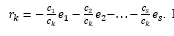
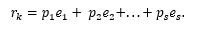
Any collection of s of linearly independent vectors in the space L forms its bases and c. This follows from the fact that any vector

r_{k}

$r_k$ linear s-dimensional vector space L can be represented in a unique way as a linear combination of basis vectors.

We fix and denote by the symbol

е_{i}

$_i$ , i = 1 (1) s, is one of the collections forming a basis of the space L. Then

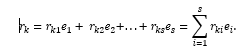
The numbers r _ki , i = 1 (1) s are called the coordinates of the vector

r_{k}

$r_k$ in the basis

е_{i}

$_i$ , i = 1 (1) s, and r _ki = (

е_{i}

$_i$ ,

r_{k}

$r_k$ ).

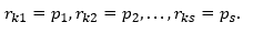
Let us show the uniqueness of the representation

r_{k}

$r_k$ ... Obviously, the set

e_{1}, e_{2}, . . ., e_{s}

$e_1,e_2,...,e_s$ ,

r_{k}

$r_k$ is dependent, since

е_{i}

$_i$ , i = 1 (1) s is a basis. In other words, there are such

с_{1}, с_{2} . . . с_{s}, c_{k}

$_1, _2... _s, c_k$ not simultaneously equal to zero, that

c_{1} \cdot e_{1} + c_{2} \cdot e_{2} + . . . + c_{s} \cdot e_{s} + c_{k} \cdot r_{k} = 0

$c_1·e_1 + c_2·e_2 + ...+ c_s·e_s + c_k·r_k = 0$ ...

Moreover, let

c_{k} \neq 0

$c_k ≠ 0$ because if

c_{k} = 0

$c_k = 0$ , then at least one of

с_{1}, с_{2}, . . ., с_{s}

$_1, _2 , ... , _s$ , it would be nonzero and then vectors

e_{i}

$e_i$ , i = 1 (1) s, would be linearly dependent, which is impossible, since this is a basis. Consequently,

Assuming

, we will have

Using the method of proof "by contradiction", we assume that the written representation

r_{k}

$r_k$ not the only one in this basis and there is something else

Then we write down the difference of representations, which, of course, is expressed as

Obviously, the right and left sides are equal, but the left one represents the difference of the vector with itself, that is, it is equal to zero. Consequently, the right-hand side is also zero. Vectors

е_{i}

$_i$ , i = 1 (1) s are linearly independent, so all the coefficients for them can only be zero. From this we get that

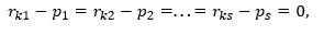
and this is possible only for

The choice of the basis. Orthonormality

Vectors are called normalized if the length of each of them is equal to one. This can be achieved by applying the normalization procedure to arbitrary vectors.

Vectors are called orthogonal if they are perpendicular to each other. Such vectors can be obtained by applying an orthogonalization procedure to each of them. If both properties are satisfied for a set of vectors, then the vectors are called orthonormal.

The need to consider orthonormal bases is caused by the need to use fast transformations of both one - and multidimensional functions. The tasks of such processing arise in the study of codes encoding information messages in communication networks of various purposes, in the study of images obtained

through automatic and automated devices, in a number of other areas using digital representations of information.

Definition. The collection of n linearly independent vectors of an n-dimensional vector

space V is called its basis.

Theorem . Each vector x of a linear n-dimensional vector space V can be represented, moreover, in a unique way, in the form of a linear combination of basis vectors. The vector space V over the field F has the following properties:

0 x = 0 (0 on the left-hand side of the equality is a neutral element of the additive group of the field F; 0 on the right-hand side of the equality is an element of the space V, which is a neutral unit element of the additive group V, called the zero vector );

(- 1) · x = –x; –1є F; x є V; –X є V;

If α x = 0єV, then for x ≠ 0 always α = 0.

Let Vn (F) be the set of all sequences (x1, x2, ..., xn) of length n with components from the field F, that is, Vn (F) = {x, such that x = (x1, x2, ..., xn), xi є F;

i = 1 (1) n}.

Addition and multiplication by a scalar are defined as follows:

x + y = (x1 + y1, x2 + y2,…, xn + yn);

α x = (α x1, α x2,…, α xn), where y = (y1, y2,…, yn),

then Vn (F) is a vector space over the field F.

Example 4 . In the vector space r = 00000, r1 = 10101, r2 = 11010, r3 = 10101 over the field F2 = {0,1} determine its dimension and basis.

Decision. Let's form a table of addition of vectors of a linear vector space

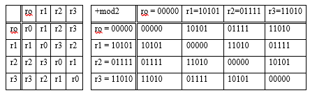
In this vector space V = {ro, r1, r2, r3} each vector has itself as its opposite. Any two vectors, excluding r, are linearly independent, which is easy to verify

c1 · r1 + c2 · r2 = 0; c1 r1 + c3 r3 = 0; c2 r2 + c3 r3 = 0;

Each of the three relations is valid only for simultaneous zero values of the pairs of coefficients ci, cj є {0,1}.

When three nonzero vectors are considered simultaneously, one of them is always the sum of the other two or is equal to itself, and r1 + r2 + r3 = r.

Thus, the dimension of the considered linear vector space is equal to two s = 2, d (L) = s = 2, although each of the vectors has five components. The basis of the space is the collection (r1, r2). You can use the pair (r1, r3) as a basis.

Theoretically and practically, the question of describing the vector space is important. It turns out that any set of basis vectors can be viewed as rows of some matrix G, called the generating matrix of the vector space. Any vector of this space can be represented as a linear combination of rows of the matrix G ( as, for example, here ).

If the dimension of the vector space is equal to k and is equal to the number of rows of the matrix G, the rank of the matrix G, then obviously there are k coefficients with q different values for generating all possible linear combinations of matrix rows. Moreover, the vector space L contains q ^k vectors.

The set of all vectors from ℤpn with operations of addition of vectors and multiplication of a vector by a scalar from ℤp is a linear vector space.

Definition . A subset W of a vector space V satisfying the conditions:

If w1, w2 є W, then w1 + w2 є W,

For any α є F and w є W, the element αw є W is

itself a vector space over the field F and is called a subspace of the vector space V.

Let V be a vector space over a field F and a set W ⊆ V. A set W is a subspace of V if W with respect to linear operations defined in V is a linear vector space.

Table. Characteristics of vector spaces

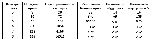
The compactness of the matrix representation of a vector space is obvious. For example, specifying L vectors of 50-bit binary numbers, among which 30 vectors form the basis of the vector space, requires the formation of the matrix G [30,50], and the described number of vectors exceeds 10 ⁹ , which seems unreasonable in the element-wise notation.

All bases of any space L are divided by the subgroup P of nondegenerate matrices with det G> 0 into two classes. One of them (arbitrarily) is called a class with positively oriented bases (right ones), the other class contains left bases.

In this case, they say that an orientation is given in space. After that, any basis is an ordered set of vectors.

If the numbering of two vectors is changed in the right basis, then the basis will become left. This is due to the fact that two rows are swapped in the matrix G, therefore, the determinant detG will change sign.

Norm and dot product of vectors

After solving the questions about finding the basis of a linear vector space, about the generation of all elements of this space and about the representation of any element and the vector space itself through the basis vectors, we can pose the problem of measuring in this space the distances between elements, angles between vectors, values of vector components , the lengths of the vectors themselves.

A real or complex vector space L is called a normed vector space if each vector r in it can be associated with a real number || r || - vector modulus, norm. A unit vector is a vector whose norm is equal to one. The zero vector has zero components.

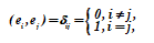
Definition... A vector space is called unitary if a binary operation is defined in it that assigns a scalar to each pair ri, rj of vectors from L. In parentheses (ri, rj) the scalar or inner product of ri and rj is written (denoted), and

1. (ri, rj) = ri ∙ rj;

2. (ri, rj) = (ri ∙ rj) *, where * indicates complex conjugation or Hermitian symmetry;

3. (ri, rj) = (ri ∙ rj) - associative law;

4. (ri + rj, rk) = (ri ∙ rk) + (rj ∙ rk) - distributive law;

5. (ri, rk) ≥ 0 and from (ri, rj) = 0 it follows ri = 0.

Definition . The positive value of the square root

is called the norm (or length, modulus) of the vector ri. If

= 1, then the vector ri is called normalized...

Two vectors ri, rj of the unitary vector space L are mutually orthogonal if their scalar product is equal to zero, i.e. (ri, rj) = 0.

For s = 3 in a linear vector space, it is convenient to choose three mutually perpendicular vectors as a basis. This choice greatly simplifies a number of dependencies and calculations. The same principle of orthogonality is used when choosing a basis in spaces and other dimensions s> 3. The use of the introduced operation of the scalar product of vectors provides the possibility of such a choice.

Even greater advantages are achieved when choosing as the basis of the vector space of orthogonal normalized vectors - the orthonormal basis... Unless otherwise stated, we will always assume that the basis ei, i = 1 (1) s is chosen in this way, i.e.

, where ij is the Kronecker symbol (1823 - 1891).

In unitary vector spaces, this choice is always realizable. Let us show the feasibility of such a choice.

Definition. Let S = {v1, v2,…, vn} be a finite subset of a vector space V over a field F.

A linear combination of vectors from S is an expression of the form a1 ∙ v1 + a2 ∙ v2 +… + an ∙ vn, where each ai ∊ F.

The envelope for the set S (notation {S}) is the set of all linear combinations of vectors from S. The envelope for S is a subspace of V.

If U is a space in V, then U is spanned by S (S contracts U) if {S} = U.

The set of vectors S is linearly dependent over F if there are scalars a1, a2, ..., an in F, not all zeros for which a1 ∙ v1 + a2 ∙ v2 +… + an ∙ vn = 0. If there are no such scalars, then the set of vectors S linearly independently over F.

If a vector space V is spanned by a linearly independent system of vectors S (or the system S contracts the space V), then the system S is called a basis for V.

Reduction of an arbitrary basis to orthonormal form

Let the space V have a non-orthonormal basis ē _i , i = 1 (1) s. We denote the norm of each basis vector by the symbol

The following statement is known [11]. If ē _i , i = 1 (1) s is an arbitrary finite or countable system of linearly independent vectors in a unitary vector space, then there exists an orthonormal system ē _i , i = 1 (1) s, generating the same linear space (manifold).

The procedure for reducing the basis to an orthonormalized form is based on the Gram - Schmidt orthogonalization process, which in turn is implemented by recurrent formulas

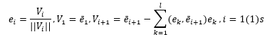
In expanded form, the basis orthogonalization and normalization algorithm contains the following conditions:

Divide the vector ē ₁ by its norm; we get the normalized vector ē _i = ē ₁ / (|| ē ₁ ||);

We form V2 = ē ₂ - (ē ₁ , ē ₂ ) e ₁ and normalize it, we get e ₂ . It is clear that then

(e1, e2) ~ (e1, e2) - (e1, e ₂ ) (e1, e1) = 0;

Constructing V3 = ē ₃ - (e1, ē ₃ ) e1 - (e2, ē ₃ ) e2 and normalizing it, we obtain e3.

For it, we immediately have (e1, e3) = (e2, e3) = 0.

Continuing this process, we obtain an orthonormal set ē _i , i = 1 (1) s. This set contains linearly independent vectors since they are all mutually orthogonal.

Let's make sure of this. Let the relation

If the set ē _i , i = 1 (1) s is dependent, then at least one cj coefficient is not equal to zero cj ≠ 0.

Multiplying both sides of the ratio by ej, we obtain

(ej, c1 ∙ e1) + (ej, c2 ∙ e2) + ... + (ej, cj ∙ ej) +… + (ej, cs ∙ rs) = 0.

Each summand in the sum is equal to zero as the scalar product of orthogonal vectors, except for (ej, cj ∙ ej), which is equal to zero in condition. But in this term

(ej, ej) = 1 ≠ 0, therefore, only cj can be zero.

Thus, the assumption that cj ≠ 0 is not true and the collection is linearly independent.

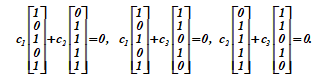
Example 5 . A basis of a 3-dimensional vector space is given:

{<-1, 2, 3, 0>, <0, 1, 2, 1>, <2, -1, -1,1>}.

The dot product is defined by the relation:

(<x1, x2, x3, x4>, <y1, y2, y3, y4>) = x1 ∙ y1 + x2 ∙ y2 + x3 ∙ y3 + x4 ∙ y4.

Using the Gram - Schmidt orthogonalization procedure, we obtain a system of vectors:

a1 = <-1, 2, 3, 0>; a2 = <0, 1, 2, 1> -4 <-1, 2, 3.0> / 7 = <4, -1, 2, 7> / 7;

a3 = <2, -1, -1, 1> + ½ <-1, 2, 3, 0> - <4, -1, 2, 7> / 5 = <7, 2, 1, -4> / ten.

(a1, a2) = (1 + 4 + 9 + 0) = 14;

a1 ^E = a1 / √14;

a2- (a1 ^E , a2) ∙ a1 ^E = a2- (8 / √14) (a1 / √14) = a2 - 4 ∙ a1 / 7;

The reader is invited to process the third vector independently.

The normalized vectors take the form:

a1 ^E = a1 / √14;

a2 ^E = <4, -1, 2, 7> / √70;

a3 ^E = <7, 2, 1, -4>/ √70;

Below, in example 6, a detailed detailed process of calculating the derivation of an orthonormal basis from a simple one (taken at random) is given.

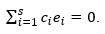
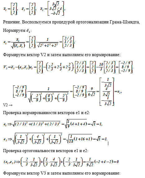
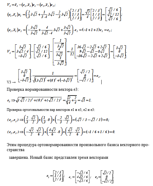
Example 6 . Reduce the given basis of the linear vector space to orthonormal form.

Given: basis vectors

Subspaces of vector spaces

Vector space structure

Representation of objects (bodies) in multidimensional spaces is a very difficult task. So, a four-dimensional cube has ordinary three-dimensional cubes as its faces, and an unfolding of a four-dimensional cube can be built in three-dimensional space. To some extent, the "imagery" and clarity of an object or its parts contributes to its more successful study.

The foregoing allows us to assume that vector spaces can be dismembered in some way, to single out parts in them called subspaces. Obviously, consideration of multidimensional and especially infinite-dimensional spaces and objects in them deprives us of the clarity of representations, which makes it very difficult to study objects in such

spaces. Even seemingly simple questions such as the quantitative characteristics of the elements of polyhedra (the number of vertices, edges, faces, etc.) in these spaces are far from completely solved.

A constructive way of studying such objects is to select their elements (for example, edges, faces) and describe them in spaces of lower dimension. So a four-dimensional cube has ordinary three-dimensional cubes as its faces, and an unfolding of a four-dimensional cube can be built in three-dimensional space. To some extent, the

"imagery" and clarity of the object or its parts contributes to their more successful study.

If L is an extension of the field K, then L can be regarded as a vector (or linear) space over K. The elements of the field L (that is, vectors) form an abelian group by addition. Moreover, each “vector” a є L can be multiplied by a “scalar” r є K, and the product ra again belongs to L (here ra is simply the product in the sense of the field L operation of the elements r and a of this field). The laws are also fulfilled

r ∙ (a + b) = r ∙ a + r ∙ b, (r + s) ∙ a = r ∙ a + r ∙ s, (r ∙ s) ∙ a = r ∙ (s ∙ a) and 1 ∙ a = a, where r, s є K, a, b є L.

The foregoing allows us to assume that vector spaces can be dismembered in some way, to single out parts in them, called subspaces. Obviously, the main result of this approach is to reduce the dimension of the allocated subspaces. Let the subspaces L1 and L2 be distinguished in a vector linear space L. As a basis for L1, a smaller set ei, i = 1 (1) s1, s1 <s, is chosen than in the original L.

The remaining basis vectors generate another subspace L2, called the “orthogonal complement” of the subspace L1. We will use the notation L = L1 + L2. It does not mean that all vectors of the space L belong to either L1 or L2, but that any vector from L can be represented as the sum of a vector from L1 and an orthogonal vector from L2.

It is not the set of vectors of the vector space L that is split, but the dimension d (L) and the set of basis vectors. Thus, the subspace L1 of a vector space L is the set L1 of its elements (of lower dimension), which itself is a vector space with respect to the operations of addition and multiplication by a number introduced in L.

Each linear vector subspace Li - contains a zero vector and, together with any of its vectors, also contains all their linear combinations. The dimension of any linear subspace does not exceed the dimension of the original space itself.

Example 7.In ordinary three-dimensional space, subspaces are all straight lines (dimension s = 1) lines, planes (dimension s = 2) passing through the origin. In the space n of polynomials of degree at most n, subspaces are, for example, all k for k <n, since adding and multiplying by numbers polynomials of degree at most k, we will again obtain the same polynomials.

However, each of the spaces Pn is contained as subspaces in the space P of all polynomials with real coefficients, and this latter is a subspace of the space C of continuous functions.

Matrices of the same type over the field of real numbers also form a linear vector space, since they satisfy all the axioms of vector spaces. The vector space L2 of sets of length n, each of which is orthogonal to the subspace L1 of sets of length n, forms a subspace L2, called the zero space for L1. In other words, each vector from L2 is orthogonal to each vector from L1 and vice versa.

Both subspaces L1 and L2 are subspaces of the vector space L of sets of length n. In coding theory [4], each of the subspaces L1 and L2 generates a linear code dual to the code generated by other subspaces. If L1 is an (n, k) -code, then L2 is an (n, n - k) -code. If a code is a vector space of rows of some matrix, then its dual code is the zero space of this matrix and vice versa.

An important issue in the study of vector spaces Vn is the establishment of their structure (structure). In other words, of interest are elements, their collections (subspaces of dimension 1 <k <n), as well as their relationships (ordering, nesting, etc.). We assume that a given vector space Vn over a finite field GF (q) formed by q = p r elements, where p is a prime number and r is an integer.

The following results are known.

The number of subspaces of a vector space

Let us give the following justification. Each vector v1 ≠ 0 from a system of k linearly independent (v1, v2,…, vk) vectors can be chosen in q ⁿ - 1 ways. The next vector v2 ≠ 0 cannot be expressed linearly in terms of v1, i.e. can be chosen in q ⁿ - q ways, etc.

The last vector vk ≠ 0 is also not linearly expressed in terms of the previously selected vectors v1, v2,…, vk and, therefore, can be chosen in q ⁿ - q ^k - 1 ways. The total number of ways to select a set of vectors v1, v2, ..., vk, thus, is defined as the product of the number of selections of individual vectors, which gives formula (1). For the case when k = n, we have w = wn, n and from formula (I) we obtain formula (2).

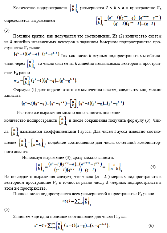
Important generalizing results on the dimensions of subspaces.

The collection of all tuples of length n orthogonal to the subspace V1 of tuples of length n forms the subspace V2 of tuples of length n. This subspace V2 is called the null space for V1.

If a vector is orthogonal to each of the vectors generating the subspace V1, then this vector belongs to the zero space for V1.

An example of (V1) is the set of 7-bit vectors of the generating matrix of the (7,4) Hamming code, with a zero subspace (V2) of 7-bit vectors that form the parity-check matrix of this code.

If the dimension of the subspace (V1) of sets of length n is equal to k, then the dimension of the zero subspace (V2) is equal to n - k.

If V2 is a subspace of tuples of length n and V1 is a zero space for V2, then (V2) is a zero space for V1.

Let U∩V denote the collection of vectors belonging to both U and V, then U∩V is a subspace.

Let U⊕V denote the subspace consisting of the collection of all linear combinations of the form a u + b v , where u є U, v є V, ab are numbers.

The sum of the dimensions of the subspaces U∩V and U⊕V is equal to the sum of the dimensions of the subspaces U and V.

Let U2 be the zero subspace for U1 and V2 the zero space for V1. Then U2∩V2 is the zero space for U1⊕V1.

Conclusion

The paper considers the basic concepts of vector spaces, which are often used in the construction of models for the analysis of encryption, coding and steganographic systems, processes occurring in them. So in the new American encryption standard, affine spaces are used, and in digital signatures on elliptic curves, both affine and

projective spaces (to speed up the processing of curve points).

We are not talking about these spaces in the work (you cannot lump everything in one heap, and I also limit the volume of publication), but the mention of this is not made in vain. Authors writing about means of protection, about cipher algorithms, naively believe that they understand the details of the described phenomena, but the understanding of Euclidean spaces and their properties is transferred without any reservations to other spaces, with different properties and laws. The reading audience is misled about the simplicity and accessibility of the material.

A false picture of reality is created in the field of information security and special equipment (technology and mathematics).

In general, I made the initiative, how fortunate the readers are to judge.

Literature

1. Avdoshin S.M., Nabebin A.A. Discrete Math. Modular algebra, cryptography, coding. - M .: DMK Press, 2017.-352 p.

2. Akimov O.E. Discrete mathematics. Logic, groups, graphs - Moscow: Lab. Base. Zn., 2001.-352 p.

3. Anderson D.A. Discrete mathematics and combinatorics), Moscow: Williams, 2003, 960 p.

4. Berlekamp E. Algebraic coding theory. -M .: Mir, 1971.- 478 p.

5. Vaulin A.E. Discrete mathematics in computer security problems. H 1- SPb .: VKA im. A.F. Mozhaisky, 2015.219 p.

6. Vaulin A.E. Discrete mathematics in computer security problems. H 2- SPb .: VKA im. A.F. Mozhaisky, 2017.-151 p.

7. Gorenstein D. Finite simple groups. Introduction to their classification.-M .: Mir, 1985.- 352 p.

7. Graham R., Knut D., Ptashnik O. Concrete mathematics. Foundations of informatics.-M .: Mir, 1998.-703 p.

9. Elizarov V.P. End rings. - M .: Helios ARV, 2006. - 304 p.

Ivanov B.N. Discrete mathematics: algorithms and programs-M .: Lab.Baz. Knowledge., 2001.280 p.

10. Yerusalimsky Ya.M. Discrete mathematics: theory, problems, applications-M .: Vuzovskaya kniga, 2000.-280 p.

11. Korn G., Korn T. Handbook of mathematics for scientists and engineers.-M .: Nauka, 1973.-832 p.

12. Lidl R., Niederreiter G. Finite fields: In 2 volumes.Vol. 1 -M .: Mir, 1988. - 430 p.

13. Lidl R., Niederreiter G. Finite fields: In 2 volumes.Vol. 2 -M .: Mir, 1988. - 392 p.

14. Lyapin E.S., Aizenshtat A.Ya., Lesokhin M.M., Exercises on the theory of groups.- Moscow: Nauka, 1967.-264 p.

15. Mutter V.M. Fundamentals of anti-jamming information transmission. -L. Energoatomizdat, 1990, 288 p.

16. Nabebin A.A. Discrete mathematics .- M .: Lab. Base. Knowledge., 2001.280 p.

17. Novikov F.A. Discrete mathematics for programmers.- SPb .: Peter, 2000.-304 p.

18. Rosenfeld B.A. Multidimensional spaces.-M .: Nauka, 1966.-648 p.

18. Hall M. The theory of groups.-M .: Izd. IL, 1962.- 468 p.

19. Shikhanovich Yu.A. Groups, rings, lattices. - SPb .: Kirtsideli, 2006. - 368 p.

20. Shneperman L.B. The course of algebra and number theory in problems and exercises: In 2 hours Part 2.-Mn .: Vysh. shk., 1987.-256 p.

21. Shneperman LB Collection of problems in algebra and number theory. - Minsk: Design PRO, 2000. -240 p.

Vector spaces