To understand how B-tree indexes came to be, let's imagine a world without them and try to solve a typical problem. Along the way, we will discuss the problems that we will face and ways to solve them.

Introduction
In the world of databases, there are two most common ways of storing information:
- Based on Log based structures.
- Based on pages.
The advantage of the first method is that it allows you to easily and quickly read and save data. New information can only be written to the end of the file (sequential recording), which ensures high recording speed. This method is used by such bases as Leveldb, Rocksdb, Cassandra.
The second method (page-based) splits the data into fixed-size chunks and saves it to disk. These parts are called "pages" or "blocks". They contain records (rows, tuples) from tables.
This method of data storage is used by MySQL, PostgreSQL, Oracle and others. And since we are talking about indexes in MySQL, this is the approach we will consider.
Data storage in MySQL
So, all data in MySQL is saved to disk as pages. The page size is regulated by the database settings and is 16 KB by default.
Each page contains 38 bytes of headers and an 8-byte ending (as shown in the figure). And the space allocated for data storage is not completely filled up, because MySQL leaves empty space on each page for future changes.
Further in the calculations, we will neglect the service information, assuming that all 16 KB of the page are filled with our data. We will not go deep into the organization of InnoDB pages, this is a topic for a separate article. You can read more about this here .

Since we agreed above that indexes do not exist yet, for example, we will create a simple table without any indexes (in fact, MySQL will still create an index, but we will not take it into account in the calculations):
CREATE TABLE `product` (
	`id` INT NOT NULL AUTO_INCREMENT,
	`name` CHAR(100) CHARACTER SET utf8 COLLATE utf8_general_ci NOT NULL,
	`category_id` INT NOT NULL,
	`price` INT NOT NULL,
) ENGINE=InnoDB;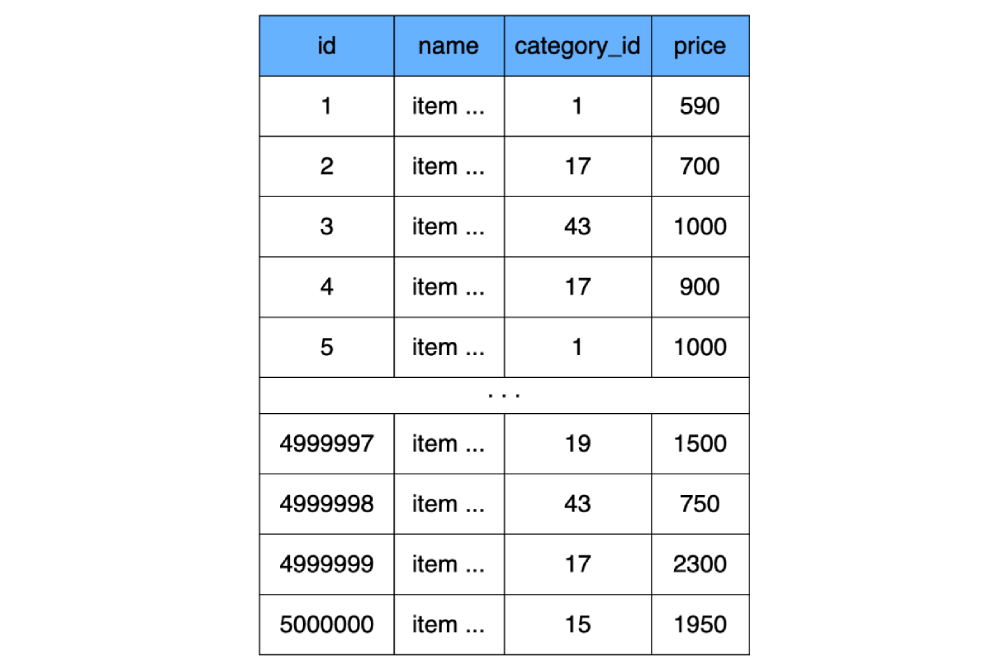
and execute the following request:
SELECT * FROM product WHERE price = 1950;MySQL will open the file where the data from the table is stored
productand begin to iterate over all the records (rows) in search of the required ones, comparing the field pricefrom each found row with the value in the query. For clarity, I specifically consider the option with a full scan of the file, so the cases when MySQL receives data from the cache are not suitable for us.
What problems can we face with this?
HDD
Since we have everything stored on a hard drive, let's take a look at its device. The hard disk reads and writes data in sectors (blocks). The size of such a sector can be from 512 bytes to 8 KB (depending on the disk). Several consecutive sectors can be combined into clusters.
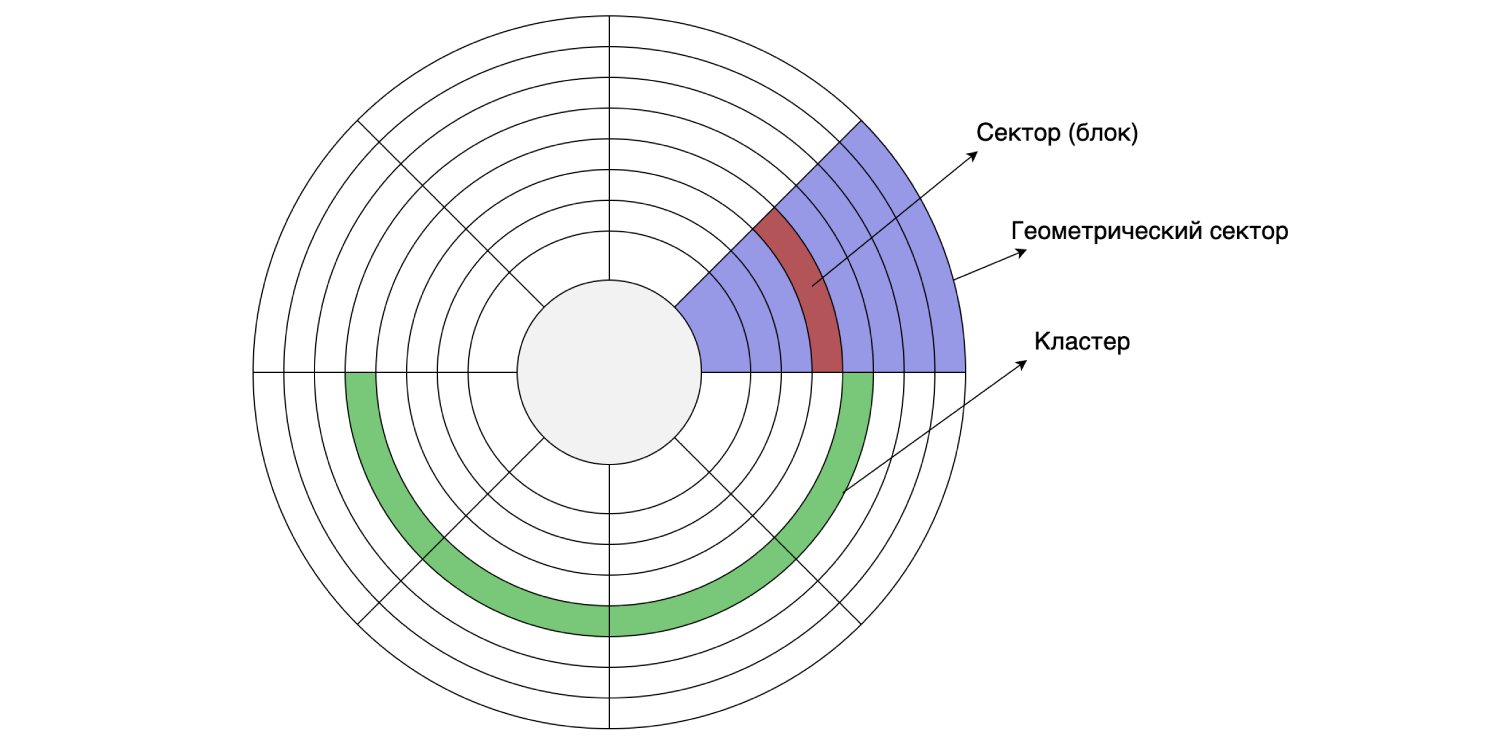
The cluster size can be set when formatting / partitioning the disk, that is, it is done programmatically. Suppose the disk sector size is 4 KB and the file system is partitioned with a 16 KB cluster size: one cluster consists of four sectors. As we remember, MySQL by default stores data on disk in 16 KB pages, so one page fits into one disk cluster.
Let's calculate how much space our product plate will take up, assuming it stores 500,000 items. We have three four-byte fields
id, priceand category_id. Let's agree that the name field for all records is filled to the end (all 100 characters), and each character takes 3 bytes. (3 * 4) + (100 * 3) = 312 bytes - this is how much one row of our table weighs, and multiplying this by 500,000 rows we get the table weight of product156 megabytes.
Thus, to store this label, 9750 clusters are required on the hard disk (9750 pages of 16 KB).
When saving to disk, free clusters are taken, which leads to "smearing" of clusters of one plate (file) across the entire disk (this is called fragmentation). Reading such blocks of memory randomly located on disk is called random read. This reading is slower because you have to move the hard disk head many times. To read the entire file, we have to jump all over the disk to get the required clusters.
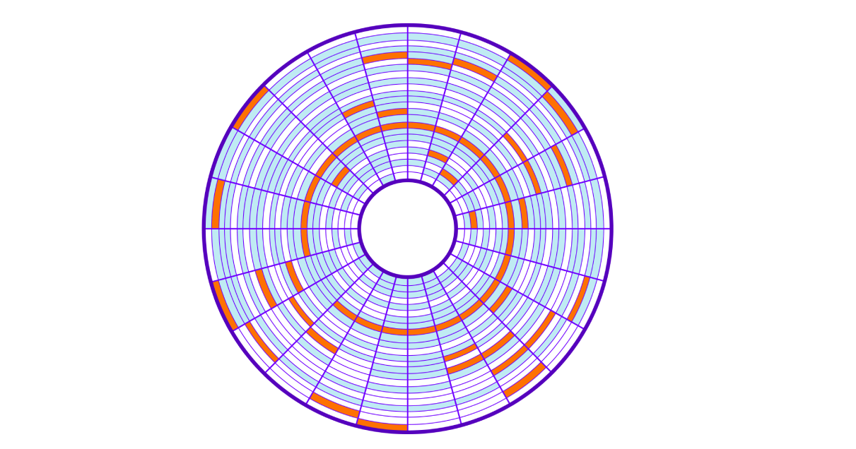
Let's go back to our SQL query. To find all the rows, the server will have to read all 9750 clusters scattered across the disk, and it will take a lot of time to move the disk read head. The more clusters we use our data, the slower it will be searched. And besides, our operation will clog the I / O system of the operating system.
In the end, we get a low read speed; "Suspend" the OS, clogging the I / O system; and do a lot of comparisons, checking the query conditions for each row.
My own bike
How can we solve this problem on our own?
We need to figure out how to improve table lookups
product. Let's create another table in which we will only store the field priceand the link to the record (area on disk) in our table product. Let's take it straight away as a rule that when adding data to a new table, we will store prices in a sorted form.
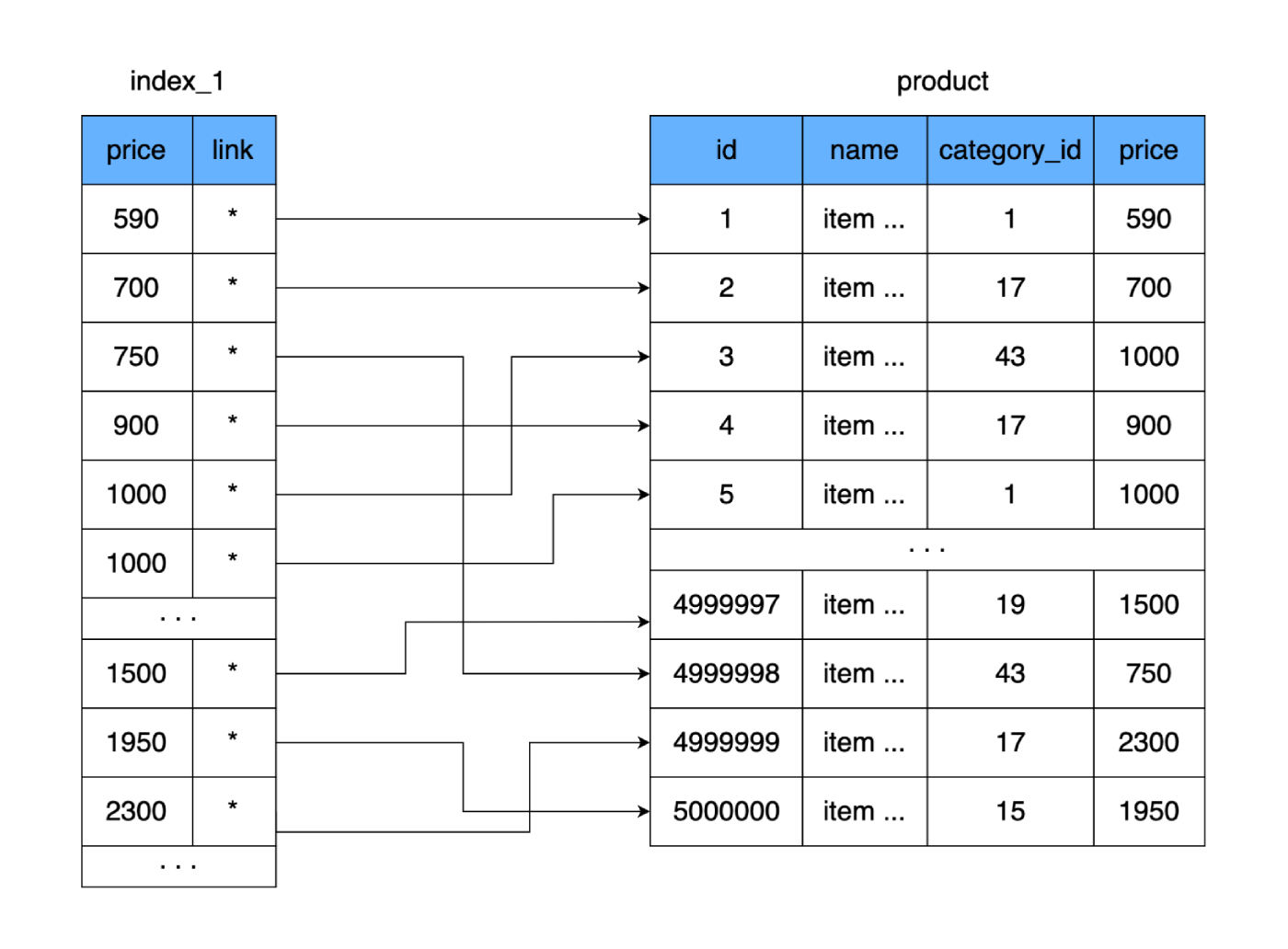
What does it give us? The new table, like the main one, is stored on the disk page by page (in blocks). It contains the price and a link to the main table. Let's calculate how much space such a table will take. The price takes 4 bytes, and let the reference to the main table (address) be 4 bytes too. For 500,000 rows, our new table will only weigh 4 MB. That way, a lot more rows from the new table will fit on one data page, and fewer pages will be needed to store all our prices.
If a complete table requires 9,750 hard disk clusters (or worst case scenario, 9,750 hard disk hops), then the new table fits only 250 clusters. Due to this, the number of used clusters on the disk will be greatly reduced, and hence the time spent on random reads. Even if we read our entire new table and compare the values to find the right price, then in the worst case, it will take 250 jumps across the clusters of the new table. And after finding the required address, we will read another cluster where the complete data is located. Result: 251 reads versus the original 9750. The difference is significant.
In addition, to search for such a table, you can use, for example, the binary search algorithm (since the list is sorted). This will save even more on the number of reads and comparison operations.
Let's call our second table an index.
Hooray! We have come up with our own
But stop: as the table grows, the index will also get bigger and bigger, and eventually we'll get back to the original problem. The search will again take a long time.
Another index
And if you create another index on top of the existing one?
Only this time we will not write down every value of the field
price, but we will associate one value with the whole page (block) from the index. That is, an additional level of index will appear, which will point to the dataset from the previous index (the page on disk where the data from the first index is stored).
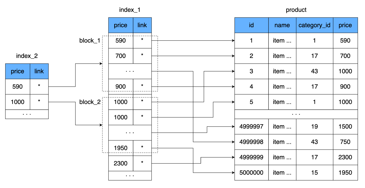
This will further reduce the number of readings. One line of our index takes 8 bytes, that is, we can fit 2000 such lines on one 16-kilobyte page. The new index will contain a link to the block of 2000 lines of the first index and the price from which this block starts. One such line also takes 8 bytes, but their number is sharply reduced: instead of 500,000, only 250. They even fit into one hard disk cluster. Thus, in order to find the required price, we will be able to determine exactly which block of 2000 lines it is in. And in the worst case, to find the same record, we:
- Let's do one read from the new index.
- After running through 250 lines, we find a link to the data block from the second index.
- Consider one cluster that contains 2000 rows with prices and links to the main table.
- Having checked these 2000 lines, we will find the required one and one more time jump across the disk to read the last data block.
We will get a total of 3 cluster jumps.
But sooner or later this level will also be filled with a lot of data. Therefore, we will have to repeat everything we have done, adding a new level over and over. That is, we need such a data structure for storing the index, which will add new levels as the size of the index grows and independently balance the data between them.
If we turn the tables over so that the last index is on top, and the main table with data is on the bottom, we get a structure very similar to a tree.
The B-tree data structure works on a similar principle, so it was chosen for these purposes.
B-trees in brief
The most common indexes used in MySQL are B-tree (balanced search tree) ordered indexes .
The general idea of a B-tree is similar to our index tables. The values are stored in order and all leaves of the tree are at the same distance from the root.
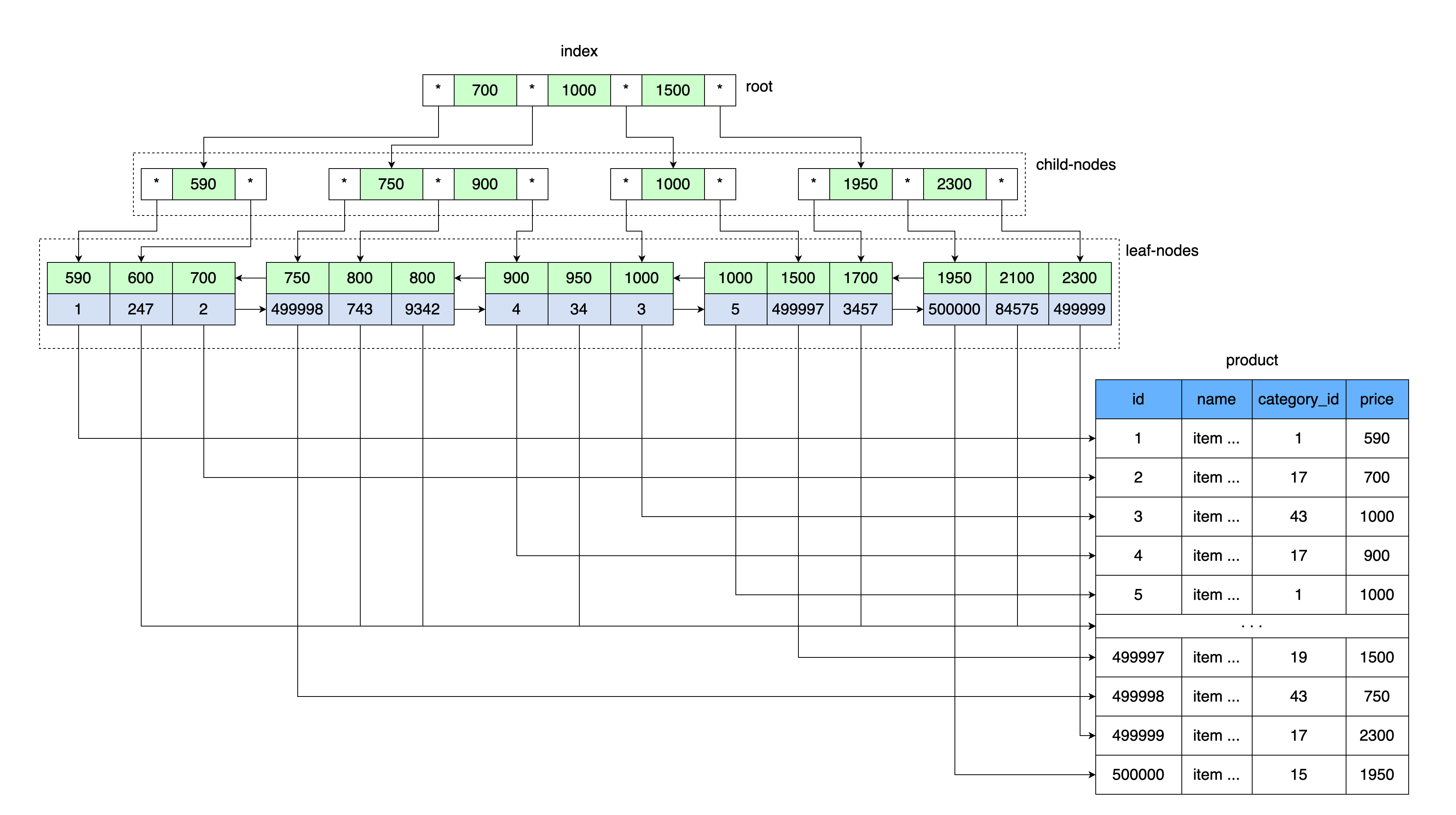
Just as our table with an index stored a price value and a link to a data block containing a range of values with this price, so the B-tree root stores a price value and a link to a memory area on disk.
First, the page that contains the root of the B-tree is read. Further, after entering the range of keys, there is a pointer to the desired child node. The page of the child node is read, from where the link to the data sheet is taken from the key value, and the page with the data is read from this link.
B-tree in InnoDB
More specifically, InnoDB uses a B + tree data structure.
Every time you create a table, you automatically create a B + tree, because MySQL stores such an index for the primary and secondary keys.
Secondary keys additionally store the values of the primary (cluster) key as a reference to the data row. Consequently, the secondary key grows by the size of the primary key value.
In addition, B + trees use additional links between child nodes, which increases the speed of searching over a range of values. Read more about the structure of b + tree indexes in InnoDB here .
Summing up
The b-tree index provides a great advantage when searching data over a range of values due to a manifold reduction in the amount of information read from the disk. It participates not only during search by condition, but also during sorts, joins, groupings. Read how MySQL uses indexes here .
Most of the queries to the database are just queries to find information by value or by a range of values. Therefore, in MySQL, the most commonly used index is a b-tree index.
Also, b-tree index helps with data retrieval. Since the primary key (clustered index) and the value of the column on which the non-clustered index is built (secondary key) are stored in the index leaves, this data can no longer be accessed from the main table and taken from the index. This is called the covering index. You can find more information about clustered and non-clustered indexes in this article .
Indexes, like tables, are also stored on disk and take up space. Each time you add information to the table, the index must be kept up to date, to monitor the correctness of all links between nodes. This creates an overhead in writing information, which is the main disadvantage of b-tree indexes. We sacrifice write speed to increase read speed.
- MySQL . 3-
: ,
: 2018 - blog.jcole.us/innodb
- dev.mysql.com/doc/refman/8.0/en/innodb-storage-engine.html