But how exactly does Object Tracking work? There are many Deep Learning solutions to this problem, and today I want to talk about a common solution and the math behind it.
So, in this article I will try to tell you in simple words and formulas about:
- YOLO is a great object detector
- Kalman Filters
- Mahalanobis distance
- Deep SORT
YOLO is a great object detector
Immediately you need to make a very important note that you need to remember - Object Detection is not Object Tracking. For many, this will not be news, but often people confuse these concepts. In simple words:
Object Detection is simply the definition of objects in the picture / frame. That is, an algorithm or neural network defines an object and records its position and bounding boxes (parameters of rectangles around objects). So far, there is no talk of other frames, and the algorithm works with only one.
Example:
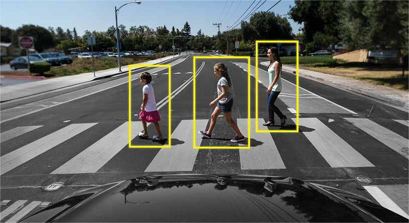
Object Tracking is another matter entirely. Here the task is not only to identify objects in the frame, but also to link information from previous frames in such a way as not to lose the object, or to make it unique.
Example:

That is, Object Tracker includes Object Detection to determine objects, and other algorithms to understand which object on a new frame belongs to which of the previous frame.
Therefore, Object Detection plays a very important role in the tracking task.
Why YOLO? Yes, because YOLO is considered more efficient than many other algorithms for identifying objects. Here is a small graph for comparison from the creators of YOLO:
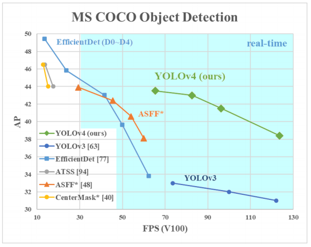
Here we are looking at YOLOv3-4 as they are the most recent versions and are more efficient than the previous ones.
Architectures of different Object Detectors
So, there are several neural network architectures designed to define objects. They are generally categorized into "two-tier" such as RCNN, fast RCNN and faster RCNN, and "single-tier" such as YOLO.
The "two-tier" neural networks listed above use the so-called regions in the picture to determine if a particular object is in that region.
It usually looks like this (for a faster RCNN, which is the fastest of the two tier systems listed):
- Picture / frame is fed to the input
- The frame is run through CNN to form feature maps
- A separate neural network defines regions with a high probability of finding objects in them
- Then, using RoI pooling, these regions are compressed and fed into the neural network, which determines the class of the object in the regions

But these neural networks have two key problems: they don't look at the whole picture, but only at individual regions, and they are relatively slow.
What is so cool about YOLO? The fact that this architecture does not have two problems from above, and it has repeatedly proved its effectiveness.
In general, the YOLO architecture in the first blocks does not differ much in terms of the "block logic" from other detectors, that is, a picture is fed to the input, then feature maps are created using CNN (although YOLO uses its own CNN called Darknet-53), then these feature maps are analyzed in a certain way (more on this later), giving out the positions and sizes of bounding boxes and the classes to which they belong.

But what are Neck, Dense Prediction, and Sparse Prediction?
We dealt with Sparse Prediction a bit earlier - it's just a re-iteration of how two-tier algorithms work: they define regions individually and then classify those regions.
Neck (or "neck") is a separate block, which is created in order to aggregate information from separate layers from the previous blocks (as shown in the figure above) to increase the accuracy of prediction. If you are interested in this, you can google the terms "Path Aggregation Network", "Spatial Attention Module" and "Spatial Pyramid Pooling".
And finally, what distinguishes YOLO from all other architectures is a block called (in our picture above) Dense Prediction. We will focus on it a little more, because this is a very interesting solution, which just allowed YOLO to break into the leader in the efficiency of object detection.
YOLO (You Only Look Once) carries the philosophy of looking at the picture once, and for this one viewing (that is, one run of the picture through one neural network) to make all the necessary object definitions. How does this happen?
So, at the output from the work of YOLO, we usually want this:
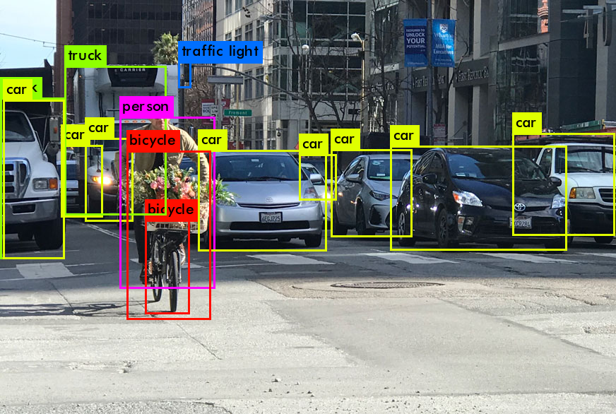
What does YOLO do when it learns from data (in simple words):
Step 1: Usually, the pictures will be reshaped to a size of 416x416 before training the neural network, so that they can be fed in batches (to speed up learning ).
Step 2: Divide the picture (for now mentally) into cells of size a x a . In YOLOv3-4, it is customary to divide into cells of 13x13 size (we will talk about different scales a little later to make it clearer).
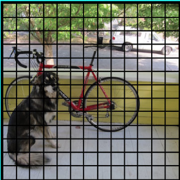
Now let's focus on these cells, into which we divided the picture / frame. These cells, called grid cells, are at the heart of the YOLO idea. Each cell is an "anchor" to which bounding boxes are attached. That is, several rectangles are drawn around the cell to define the object (since it is not clear what shape the rectangle will be most suitable, they are drawn at once in several and different shapes), and their positions, width and height are calculated relative to the center of this cell.
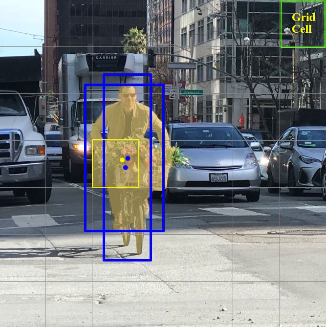
How are these bounding boxes drawn around the cage? How is their size and position determined? This is where the anchor boxes technique (in translation - anchor boxes, or "anchor rectangles") comes into play. They are set at the very beginning either by the user himself, or their sizes are determined based on the sizes of the bounding boxes that are in the dataset on which YOLO will train (K-means clustering and IoU are used to determine the most appropriate sizes). Usually, there are 3 different anchor boxes that will be drawn around (or inside) one cell:

Why is this done? It will be clear now as we discuss how YOLO learns.
Step 3. The picture from the dataset is run through our neural network (note that in addition to the picture in the training dataset, we must have the positions and sizes of the real bounding boxes for the objects on it. This is called "annotation" and is done mostly manually ).
Let's now think about what we need to get at the output.
For each cell, we need to understand two fundamental things:
- Which of the 3 anchor boxes drawn around the cage suits us best and how can we tweak it a bit so that it fits well with the object
- What object is inside this anchor box and is it there at all
What should then be the output of YOLO?
1. At the output for each cell, we want to get:

2. The output should include the following parameters:
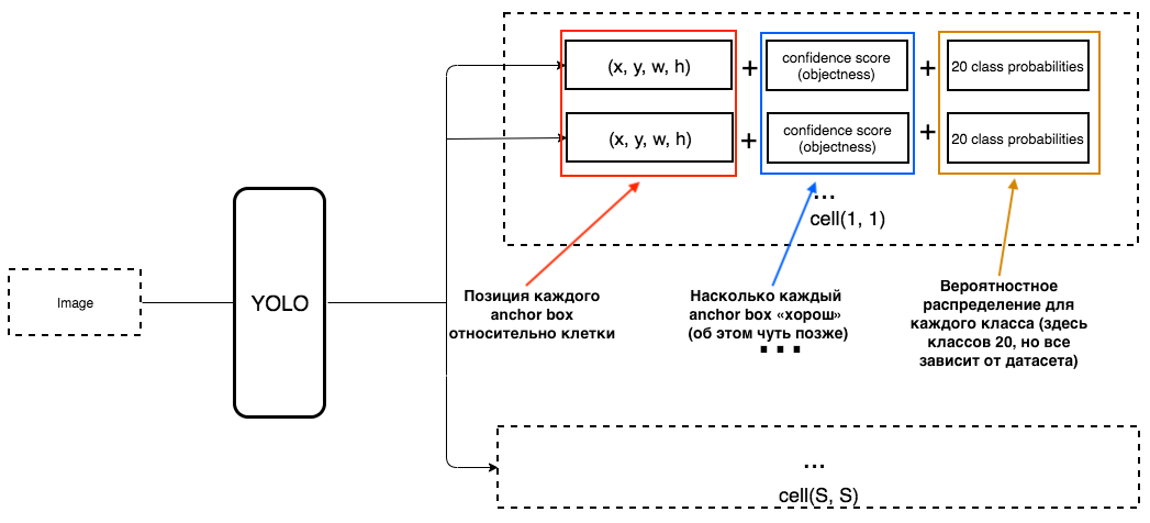
How is objectness determined? In fact, this parameter is determined using the IoU metric during training. The IoU metric works like this:

At the beginning, you can set a threshold for this metric, and if your predicted bounding box is above this threshold, then it will have objectness equal to one, and all other bounding boxes with lower objectness will be excluded. We will need this value of objectness when we calculate the overall confidence score (to what extent we are sure that this is the object we need is located inside the predicted rectangle) for each specific object.
And now the fun begins. Let's imagine that we are the creators of YOLO and we need to train her to recognize people in the frame / picture. We feed the image from the dataset to YOLO, where feature extraction occurs at the beginning, and at the end we get a CNN layer that tells us about all the cells into which we "divided" our image. And if this layer tells us a "lie" about the cells in the picture, then we must have a large Loss, so that later it can be reduced when the following pictures are fed into the neural network.
To be clear, there is a very simple diagram of how YOLO creates this last layer:
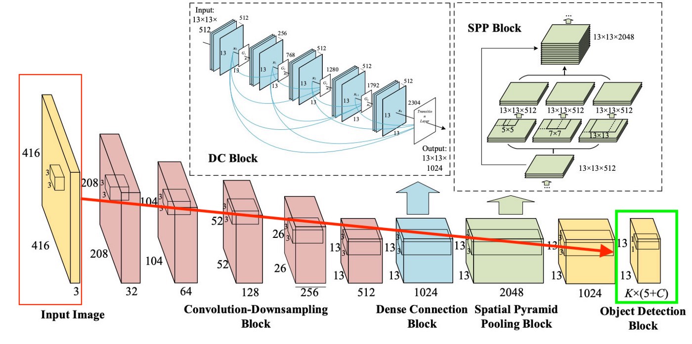
As we can see from the picture, this layer is 13x13 (for pictures, the original size is 416x416) in order to talk about "each cell" in the picture. From this last layer, the information that we want is obtained.
YOLO predicts 5 parameters (for each anchor box for a specific cell):

To make it easier to understand, there is a good visualization on this topic:

As you can understand them from this picture, YOLO's task is to predict these parameters as accurately as possible in order to determine the object in the picture as accurately as possible. And the confidence score, which is determined for each predicted bounding box, is a kind of filter in order to filter out completely inaccurate predictions. For each predicted bounding box, we multiply its IoU by the probability that this is a certain object (the probability distribution is calculated during training of the neural network), we take the best probability of all possible, and if the number after multiplication exceeds a certain threshold, then we can leave this predicted bounding box in the picture.
Further, when we have only predicted bounding boxes with a high confidence score, our predictions (if visualized) may look something like this:
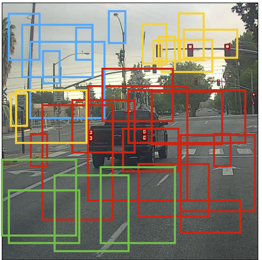
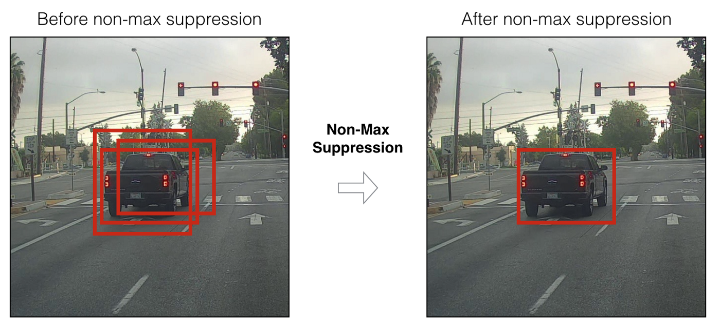
We can now use the NMS (non-max suppression) technique to filter out bounding boxes in such a way that for of one object there was only one predicted bounding box.
You should also know that YOLOv3-4 is predicted on 3 different scales. That is, the picture is divided into 64 grid cells, into 256 cells and into 1024 cells in order to also see small objects. For each group of cells, the algorithm repeats the necessary actions during prediction / learning, which were described above.
Many techniques have been used in YOLOv4 to increase model accuracy without losing too much speed. But for the prediction itself, Dense Prediction was left the same as in YOLOv3. If you are interested in what the authors have done so magically to increase the accuracy without losing speed, there is an excellent article written about YOLOv4 .
I hope I was able to convey a little bit about how YOLO works in general (more precisely, the last two versions, that is, YOLOv3 and YOLOv4), and this will awaken in you a desire to use this model in the future, or learn a little more about its work.
Now that we have figured out what is perhaps the best neural network for Object Detection (in terms of speed / quality), let's finally move on to how we can associate information about our specific YOLO objects between video frames. How can the program understand that the person in the previous frame is the same person as in the new one?
Deep SORT
To understand this technology, you must first understand a couple of mathematical aspects - Mahalonobis distance and Kalman filter.
Mahalonobis distance
Let's look at a very simple example to intuitively understand what the Maholonobis distance is and why it is needed. Many people probably know what the Euclidean distance is. Usually, this is the distance from one point to another in Euclidean space:


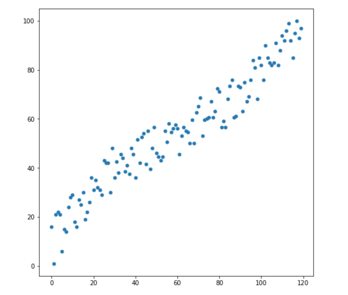
Let's say we have two variables - X1 and X2. For each of them, we have many dimensions.
Now, let's say we have 2 new dimensions:
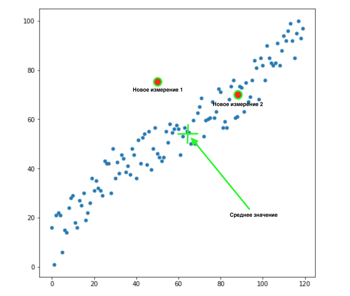
How do we know which of these two values is most appropriate for our distribution? Everything is obvious to the eye - point 2 suits us. But the Euclidean distance to the mean is the same for both points. Accordingly, a simple Euclidean distance to the mean will not work for us.
As we can see from the picture above, the variables are correlated with each other, and quite strongly. If they didn't correlate with each other, or correlated much less, we could close our eyes and apply Euclidean distance for certain tasks, but here we need to correct for the correlation and take it into account.
This is exactly what the Mahalonobis distance can handle. Since there are usually more than two variables in datasets, we will use a covariance matrix instead of correlation:

What Mahalonobis distance actually does:
- Get rid of variable covariance
- Makes the variance of variables equal to 1
- Then it uses the usual Euclidean distance for the transformed data.
Let's look at the formula for how the Mahalonobis distance is calculated:

Let's see what the components of our formula mean:
- This difference is the difference between our new point and the means for each variable
- S is the covariance matrix that we talked about a little earlier.
A very important thing can be understood from the formula. We are in fact multiplying by the inverted covariance matrix. In this case, the higher the correlation between the variables, the more likely we will shorten the distance, since we will multiply by the inverse of a larger one - that is, a smaller number (if in simple words).
We will probably not go into the details of linear algebra, all we need to understand is that we measure the distance between points in such a way as to take into account the variance of our variables and the covariance between them.
Kalman filter
To realize that this is a cool, proven thing that can be applied in so many areas, it is enough to know that the Kalman filter was used in the 1960s. Yes, yes, I am hinting at this - the flight to the moon. It has been applied there in several places, including working with round-trip flight paths. The Kalman filter is also often used in time series analysis in financial markets, in the analysis of indicators of various sensors in factories, enterprises and many other places. I hope I managed to intrigue you a little and we will briefly describe the Kalman filter and how it works. I also advise you to read this article on Habré if you want to learn more about it.
Kalman filter
, . , , .
, . 4 . , 72 .
3 :
1) (Kalman Gain):

, - ( ).
2) , ( , ), , .
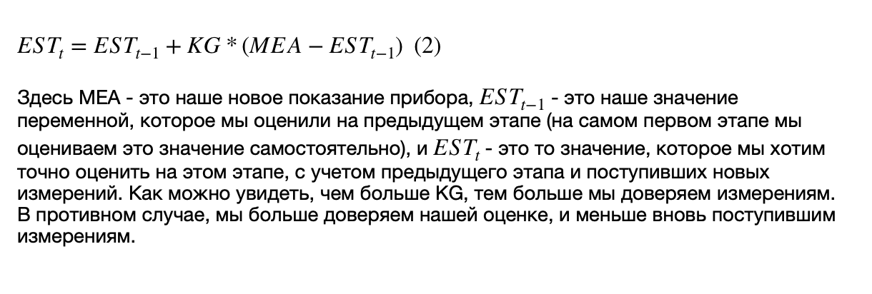
3) (), :

, :
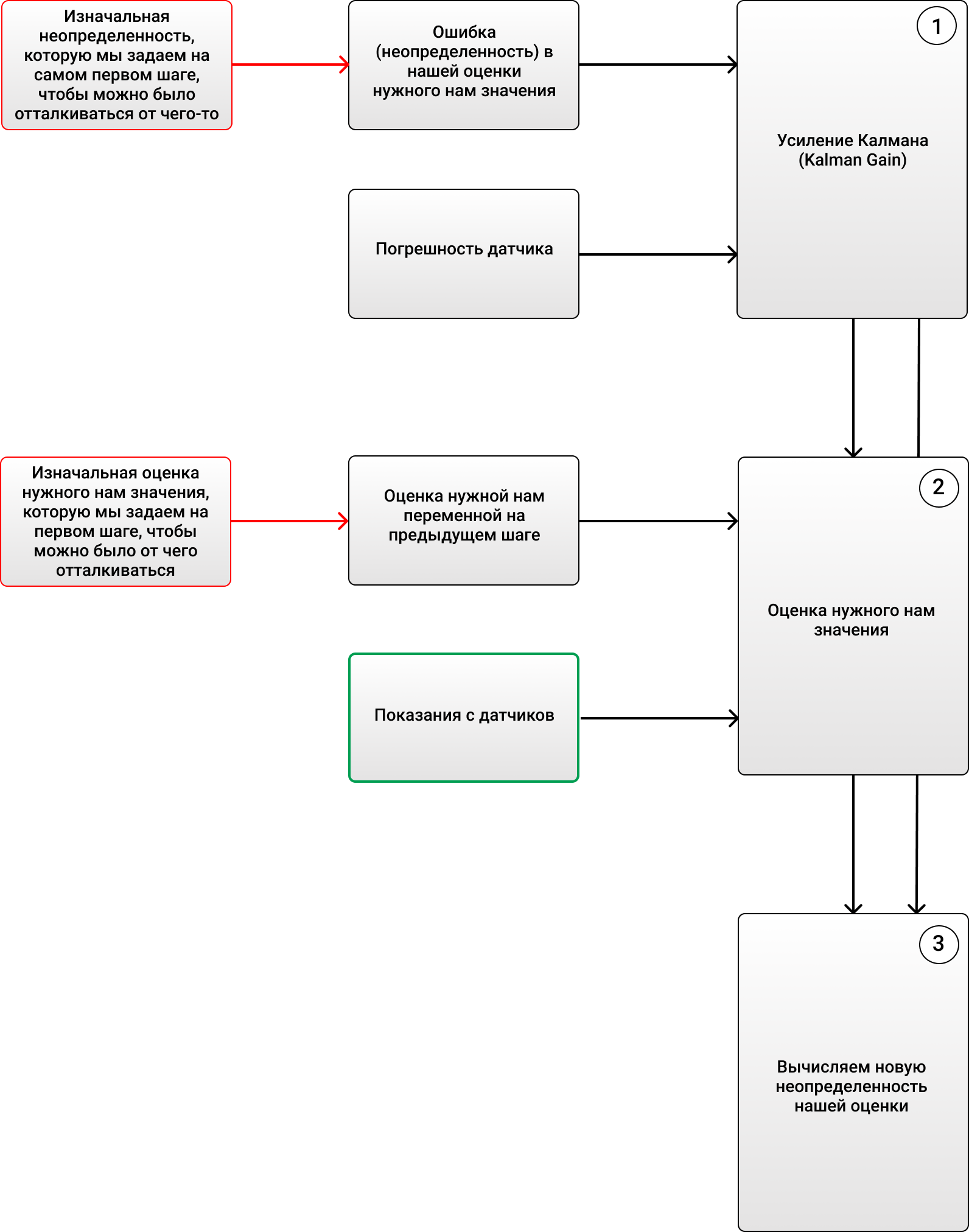
, 69 ( ), 2 . , , 4 (, , ), KG (1) 2/(2+4) = 0.33. ( ), . 70 (), . (2), , 68+0.33(70-68)=68.66. (3) (1-0.33)2 = 1.32. , , , . :
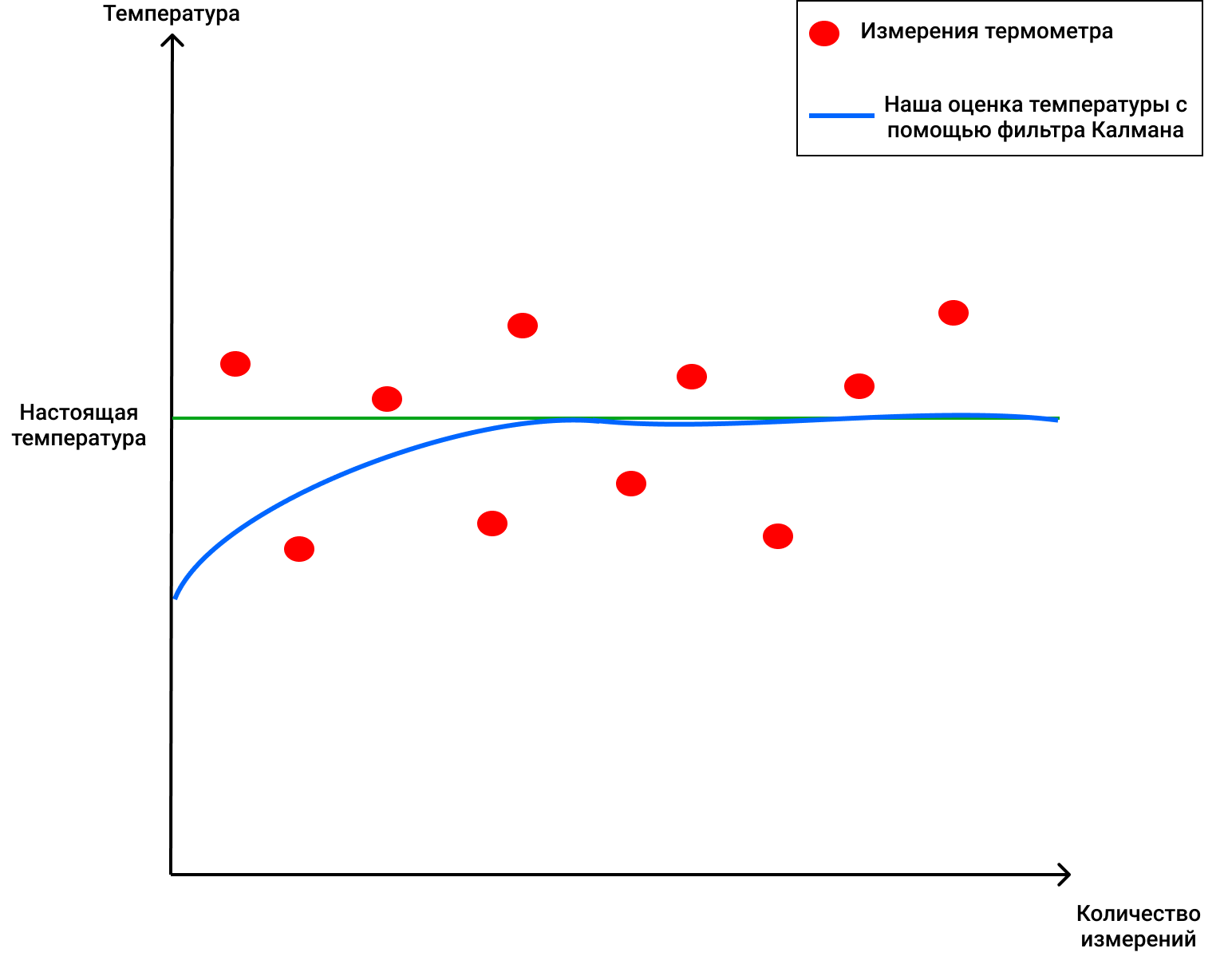
, !
, , , , , ( , ).
, . 4 . , 72 .
3 :
1) (Kalman Gain):

, - ( ).
2) , ( , ), , .

3) (), :

, :

, 69 ( ), 2 . , , 4 (, , ), KG (1) 2/(2+4) = 0.33. ( ), . 70 (), . (2), , 68+0.33(70-68)=68.66. (3) (1-0.33)2 = 1.32. , , , . :

, !
, , , , , ( , ).
DeepSORT - finally!
So, we now know what the Kalman filter and the Mahalonobis distance are. DeepSORT technology simply links these two concepts together in order to transfer information from one frame to another, and adds a new metric called appearance. First, using object detection, the position, size and class of one bounding box are determined. Then you can, in principle, apply the Hungarian algorithm to associate certain objects with object IDs that were previously on the frame and tracked using Kalman filters - and everything will be super, like in the original SORT... But the DeepSORT technology allows to improve the detection accuracy and reduce the number of switching between objects, when, for example, one person in the frame briefly obstructs another, and now the person who was obstructed is considered a new object. How does she do it?
She adds a cool element to her work - the so-called "appearance" of people who appear in the frame (appearance). This look was trained by a separate neural network that was created by the authors of DeepSORT. They used about 1,100,000 pictures from over 1000 different people to make the neural network predict correctlyThe original SORT has a problem - since the appearance of the object is not used there, then in fact, when the object covers something for several frames (for example, another person or a column inside a building), the algorithm then assigns another ID to this person - as a result whereby the so-called "memory" of objects in the original SORT is rather short-lived.
So now the objects have two properties - their dynamics of movement and their appearance. For dynamics, we have indicators that are filtered and predicted using the Kalman filter - (u, v, a, h, u ', v', a ', h'), where u, v is the X position of the predicted rectangle and Y, a is the aspect ratio of the predicted rectangle, h is the height of the rectangle, and the derivatives with respect to each value. For appearance, a neural network was trained, which had the structure:
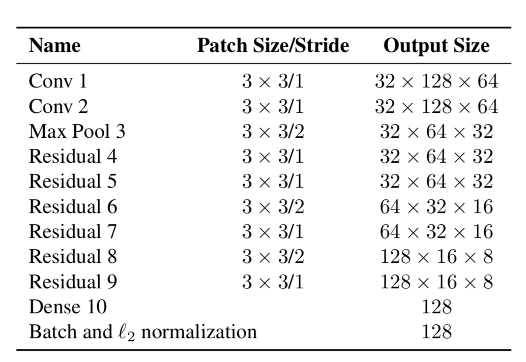
And at the end it gave out a feature vector, 128x1 in size. And then, instead of calculating the distance between certain objects using YOLO, and objects that we already followed in the frame, and then assigning a certain ID simply using the Mahalonobis distance, the authors created a new metric for calculating the distance, which includes both predictions using Kalman filters, and "cosine distance", as it is called otherwise, the Otiai coefficient.
As a result, the distance from a certain YOLO object to the object predicted by the Kalman filter (or an object that is already among those that was observed in the previous frames) is:

Where Da is the external similarity distance and Dk is the Mahalonobis distance. Further, this hybrid distance is used in the Hungarian algorithm in order to correctly sort certain objects with existing IDs.
Thus, a simple additional metric Da helped create a new, elegant DeepSORT algorithm that is used in many problems and is quite popular in the Object Tracking problem.
The article turned out to be quite weighty, thanks to those who read to the end! I hope I was able to tell you something new and help you understand how Object Tracking works on YOLO and DeepSORT.