I have always been interested in system failures and the oddities of their behavior, especially when they work in their normal conditions. I recently saw one of the slides in Ian Goodfellow's presentation, which I found very funny. A random visual noise was fed to a trained neural network, and she recognized it as one of the objects she knew. Many questions immediately arise here. Will different trained neural networks see the same object? What is the maximum level of confidence in the neural network that this random noise is indeed a recognized object? And what does the neural network actually "see" there?
Out of my curiosity about this, this record was born. Fortunately, experiments like this are very easy to do with PyTorch.... To visualize why the neural network classifies objects in a certain way, I use the Captum model interpretability framework . The code can be downloaded from Github .
Importance of questions
You may ask why these questions are important. In many cases, developers don't build models from scratch. They choose platforms and pre-trained networks from the model zoo as starting points. This saves time - there is no need to collect data and conduct initial training of the neural network. However, it also means that unexpected problems can arise in unexpected places. Depending on how this model is used, security issues can arise in the process.
Pretrained models
Pretrained models are easy to get started with and can quickly submit data for classification. In this case, you do not need to define the models and train them - all this has already been done before you, and they are ready to use immediately after deployment. Pretrained models from the Torchvision library are trained on a set of images from the Imagenet database , divided into 1000 categories... It is important to remember that this training involved identifying a single object in a picture, not parsing complex images containing various objects. In the second case, you can also get interesting results, but this is a completely different topic. Downloading pre-trained models from the Torchvision library is very easy. You just need to import the selected model by setting the pretrained parameter to True. I have also included an evaluation mode in the models, since there is no learning curve during the tests.
First I have a line of code that chooses to use cuda or cpu, depending on whether a GPU is available. For such simple tests, a GPU is not required, but since I have one, I use it.
device = "cuda" if torch.cuda.is_available() else "cpu"

import torchvision.models as models
vgg16 = models.vgg16(pretrained=True)
vgg16.eval()
vgg16.to(device)
A list of pretrained models from Torchvision can be found here . I didn't want to use all pre-trained neural networks, this is already too much. I chose the following five:
- vgg16
- resnet18
- alexnet
- densenet
- inception
I did not use any special methodology for choosing neural networks. For example, Vgg16 and Inception are often used in different examples, and they are all different.
How to create images with noise
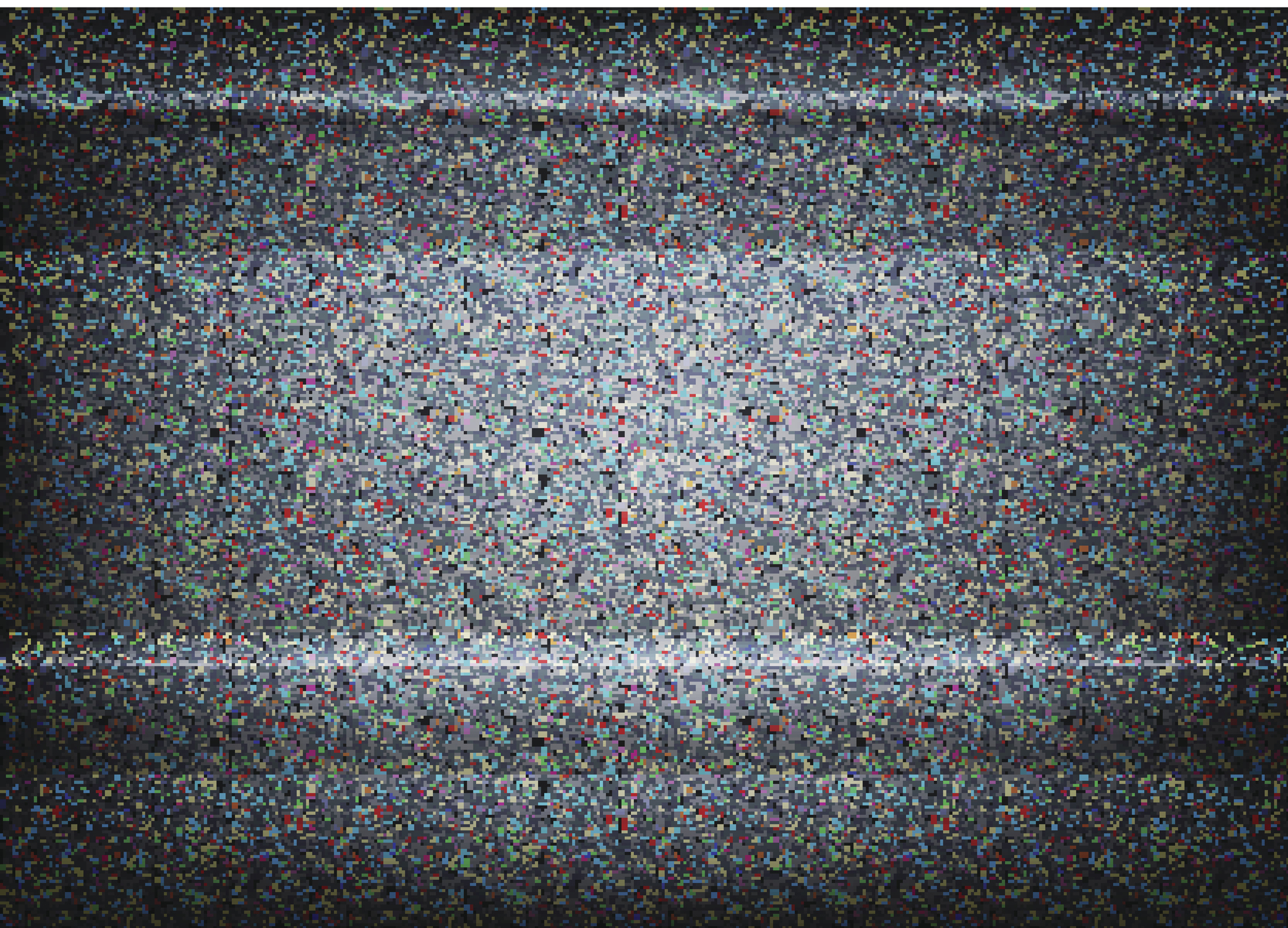
We will need a way to automatically generate images containing noise that can be fed to neural networks. To do this, I used a combination of the Numpy and PIL libraries, and wrote a small function that returns an image filled with random noise.
import numpy as np
from PIL import Image

def gen_image():
    image = (np.random.standard_normal([256, 256, 3]) * 255).astype(np.uint8)
    im = Image.fromarray(image)

    return im
You end up with something like the following:

Converting images
After that, we need to convert our images to tensor and normalize them. The following code can be used not only on random noise, but also on any image that we want to feed to pre-trained neural networks (that's why the code uses the Resize and CenterCrop values).
def xform_image(image):

    transform = transforms.Compose([transforms.Resize(256),
                                    transforms.CenterCrop(224),
                                    transforms.ToTensor(),
                                    transforms.Normalize([0.485, 0.456, 0.406],
                                                         [0.229, 0.224, 0.225])])

    new_image = transform(image).to(device)
    new_image = new_image.unsqueeze_(0)

    return new_image
We get predictions
Having prepared the transformed images, it is easy to get predictions from the unfolded model. In this case, the xform_image function is assumed to return image_xform. In the code I used for testing, I split the work between these two functions, but here I have put them together for ease of reference. We essentially need to feed the transformed image to the network, run the softmax function, use the topk function to get the score, and the predicted label ID for the best result.
with torch.no_grad():
    vgg16_res = vgg16(image_xform)
    vgg16_output = F.softmax(vgg16_res, dim=1)
    vgg16score, pred_label_idx = torch.topk(vgg16_output, 1)
results
Well, now we see how to generate noisy images and feed them to a pretrained network. So what are the results? For this test, I decided to generate 1000 noisy images, ran them through 5 selected pre-trained networks, and stuffed them into a Pandas dataframe for quick analysis. The results were interesting and somewhat unexpected.
| vgg16 | resnet18 | alexnet | densenet | inception | |
|---|---|---|---|---|---|
| count | 1000.000000 | 1000.000000 | 1000.000000 | 1000.000000 | 1000.000000 |
| mean | 0.226978 | 0.328249 | 0.147289 | 0.409413 | 0.020204 |
| std | 0.067972 | 0.071808 | 0.038628 | 0.148315 | 0.016490 |
| min | 0.074922 | 0.127953 | 0.061019 | 0.139161 | 0.005963 |
| 25% | 0.178240 | 0.278830 | 0.120568 | 0.291042 | 0.011641 |
| 50% | 0.223623 | 0.324111 | 0.143090 | 0.387705 | 0.015880 |
| 75% | 0.270547 | 0.373325 | 0.171139 | 0.511357 | 0.022519 |
| max | 0.438011 | 0.580559 | 0.328568 | 0.868025 | 0.198698 |
As you can see, some of the neural networks have decided that this noise is actually representing something specific with a fairly high level of confidence. Resnet18 and densenet have peaked at 50%. This is all good, but what exactly do these networks “see” in the noise? It is interesting that different networks "found" different objects there. Each of the networks saw something different. Resnet18 was 100% sure that it was a jellyfish, while Inception, on the contrary, had very little confidence in predictions, although at the same time she saw many more objects than any other network.
Vgg16:


 978


 14


  7


 1


Resnet18:


 1000


Alexnet:


 942


   58


Densenet:


  893


  37


 33


  20


  16


 1


Inception:


 155


 123


 102


 85


  83


  81


 69


 32


 26


 25


 24


 18


 16


 16


 12


  12


 11


  9


 9


 8


 7


 5


 5


  5


- 5


  4


 4


 4


 4


 3


 3


 3


   3


 3


 2


 2


   2


 2


  2


  1


 1


  1


 1


 1


 1


 1


 1


  1


  1


 1


 1


 1


 1


 1


 1
Just for fun, I decided to see what kind of signature Microsoft will put under the noise image, which I brought closer to the beginning of this entry. For the test, I decided to go the simplest way and used PowerPoint from Office 365. The result is interesting because unlike imagenet models that try to recognize a single object, PowerPoint tries to recognize multiple objects in order to create an accurate description of the image.
The image shows an elephant, people, big, ball.
The result did not disappoint me. From my point of view, the noise image was recognized as a circus.
Perspectives
This leads us to another question - what does the neural network see that makes it think that noise is an object? In our search for an answer, we can use a model interpretation tool that will allow us to roughly understand what the network "sees". Captum is a model interpretation framework for PyTorch. I didn't do anything special here, I just used the code from the tutorials on their website. I just added the internal_batch_size parameter with a value of 50, because without it my GPU ran out of memory very quickly.
For the renderings, I used two gradient based attributions and an occlusion based attribution. With these visualizations, we try to understand what was important to the classifier and therefore “see” what the network sees. Also I used my pre-trained resnet model, however you can change the code and use any other pre-trained models.
Before moving on to noise, I took the image of chamomile as a demonstration of the rendering process, since its signs are easy to recognize.
result = resnet18(image_xform)
result = F.softmax(result, dim=1)
score, pred_label_idx = torch.topk(result, 1)

integrated_gradients = IntegratedGradients(resnet18)
attributions_ig = integrated_gradients.attribute(image_xform, target=pred_label_idx,
                                                 internal_batch_size=50, n_steps=200)

default_cmap = LinearSegmentedColormap.from_list('custom blue',
                                                 [(0, '#ffffff'),
                                                  (0.25, '#000000'),
                                                  (1, '#000000')], N=256)

_ = viz.visualize_image_attr(np.transpose(attributions_ig.squeeze().cpu().detach().numpy(), (1,2,0)),
                             np.transpose(image_xform.squeeze().cpu().detach().numpy(), (1,2,0)),
                             method='heat_map',
                             cmap=default_cmap,
                             show_colorbar=True,
                             sign='positive',
                             outlier_perc=1)
noise_tunnel = NoiseTunnel(integrated_gradients)

attributions_ig_nt = noise_tunnel.attribute(image_xform, n_samples=10, nt_type='smoothgrad_sq', target=pred_label_idx, internal_batch_size=50)
_ = viz.visualize_image_attr_multiple(np.transpose(attributions_ig_nt.squeeze().cpu().detach().numpy(), (1,2,0)),
                                      np.transpose(image_xform.squeeze().cpu().detach().numpy(), (1,2,0)),
                                      ["original_image", "heat_map"],
                                      ["all", "positive"],
                                      cmap=default_cmap,
                                      show_colorbar=True)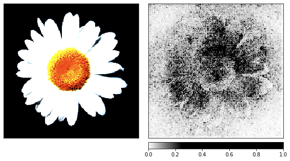
occlusion = Occlusion(resnet18)

attributions_occ = occlusion.attribute(image_xform,
                                       strides = (3, 8, 8),
                                       target=pred_label_idx,
                                       sliding_window_shapes=(3,15, 15),
                                       baselines=0)

_ = viz.visualize_image_attr_multiple(np.transpose(attributions_occ.squeeze().cpu().detach().numpy(), (1,2,0)),
                                      np.transpose(image_xform.squeeze().cpu().detach().numpy(), (1,2,0)),
                                      ["original_image", "heat_map"],
                                      ["all", "positive"],
                                      show_colorbar=True,
                                      outlier_perc=2,
                                     )

Noise visualization
We generated the previous images based on the chamomile, and now it's time to see how things work with random noise.
I am using the pretrained resnet18 network and with this image she is 40% sure she sees a jellyfish. I will not repeat the code, the code for rendering is the same as the one given above.


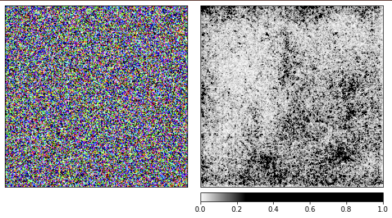

From the visualizations, it is clear that we humans will never be able to understand why the network sees a jellyfish here. Some areas of the image are marked as more important, but they are not at all as defined as we saw in the chamomile example. Unlike chamomile, jellyfish are amorphous and differ in the level of transparency.
You might be wondering what the rendering of processing a real image of a jellyfish would look like? My code is posted on Github, and it will be easy to get an answer to this question with its help.
Conclusion
Based on this recording, it's easy to see how easy it is to fool neural networks by feeding them unexpected inputs. To their credit, we will say that they did their job and gave the best result that they could. It can also be seen from the results of the work that in such cases it is not enough just to filter out options with low confidence, since some options had rather high confidence. We need to keep a close eye on situations in which real world systems fail so easily. We should not be taken aback by unexpected data entering the system - and this is what security experts have been doing for quite some time.