DIY window functions

In digital signal processing, window functions are widely used to limit the signal in time, and their names are well known to everyone who has come across the discrete Fourier transform in one way or another: Hann, Hamming, Blackman, Harris, and others. But are they sufficient, is it possible to come up with something new and is there any sense in it?



In this article, we will look at the output of a window function with new properties using Wolfram Mathematica. It is also assumed that the reader has a general understanding of digital signal processing in the context of the issue under discussion and is at least familiar with the article from Wikipedia .

Introduction

Historically, the first window functions appeared in the process of attempts to improve their spectral properties by reducing the amplitude of the side lobes - since when the signal is multiplied by the window function, their spectra are convoluted, which introduces some limitations for analysis. At that time, the 50s of the 20th century, the computing power did not allow to easily and naturally manipulate symbolic computations, and the selection of the optimal parameters was quite difficult. This is one of the reasons why the functions are called by different names - they, or rather, their spectral properties, have been studied by different researchers for quite a long time. A side effect of this is that the existing set of named window functions is perceived as a kind of "standard set" outside of which nothing can be found;at the same time, the names of these windows do not carry any information about the properties and suggest their separate study and memorization.

Classification

All window functions are obtained by multiplying some function by a rectangular one, which is guaranteed to ensure its time constraint. Therefore, first of all, they can be classified according to the functions that they use:

1. the sum of the cosines. The most extensive class due to the fact that their spectrum is easily computable and is the sum of weighted sinc functions. This includes Hann, Hamming, Blackman, Harris ...
2. piecewise continuous polynomial. They are obtained as a result of convolution of simple functions - for example, rectangular and triangular. At the same time, their spectra are multiplied and their finding is also not particularly difficult. These include Dirichlet, Triangular, Parzen, Welch ...
3. all others - using exponentials, Gaussians, sinc and others, the choice of specific functions in which is more ideological in nature than specifically spectral properties.

They can also be divided by properties at the edges:

1. no gaps at the edges - values ​​equal to zero. Breaks are of Dirichlet, Hamming, Blackman-Harris. Don't have - Triangular, Hann, Nuttal
2. absence of discontinuities of the 1st and other derivatives

Two more window functions stand out separately:

1. Kaiser, which allows you to set the width of the main petal;
2. Dolph-Chebyshev, all side lobes of which are equal to a given amplitude.

Both of them have discontinuities at the edges of both values ​​and derivatives, and their calculations involve some difficulties - the Kaiser function is calculated through a special function (Bessel), and the Dolph-Chebyshev function is determined in the frequency domain and is calculated through the inverse discrete Fourier transform. Finding their analytical antiderivatives is also particularly difficult.

Reverse engineering

Let's look at the definitions of the Blackman and Nuttel functions:

BlackmanWindow[x] // FunctionExpand

↓

$$

$$\left\{ \begin{array}{ll} \frac{1}{50} (25 \cos (2 \pi x)+4 \cos (4 \pi x)+21) & -\frac{1}{2}\leq x\leq \frac{1}{2} \\ 0 & \left| x\right| >\frac{1}{2} \\ \end{array} \right.$$

NuttallWindow[x] // FunctionExpand

↓

$$

$$\left\{ \begin{array}{ll} \frac{121849 \cos (2 \pi x)+36058 \cos (4 \pi x)+3151 \cos (6 \pi x)+88942}{250000} & -\frac{1}{2}\leq x\leq \frac{1}{2} \\ 0 & \left| x\right| >\frac{1}{2} \\ \end{array} \right.$$

They are sums of 3 and 4 cosine waves with even frequencies (starting from zero) and some coefficients. Where did these coefficients come from? It is unlikely that they were selected by hand, at least each separately - after all, there are boundary conditions that the windows must comply with regardless of their spectral properties - at least equal to unity in the center.



Let's try to "invent" the Blackman function on our own. To do this, we define a function with as yet unknown coefficients

f = Function[x, a + b Cos[2 Pi x] + c Cos[4 Pi x]];

and compose a system of equations defining the boundary conditions - equality to unity at the center, zero at the edges, and equality to zero of derivatives at the edges:

ss = Solve[{
   f[0] == 1,
   f[1/2] == 0,
   f'[1/2] == 0
   }, {a, b, c}]

↓

$$

$$\left\{\left\{b\to \frac{1}{2},c\to \frac{1}{2}-a\right\}\right\}$$

The solution was found, but not one, but many - depending on the coefficient a , which Wolfram politely warned us about. Now, from the found solution, we define a new function depending on the unknown coefficient: ↓ It is easy to see that for a = 0.42 we obtain the Blackman function. But why exactly 0.42? To answer this question, we need to plot its spectrum. Analytical Fourier Transform is not an easy task, but Wolfram can handle it too, saving us from the chore.



hx = Function[{x, a},

Piecewise[{{f[x] /. ss[[1]], -1/2 < x < 1/2}}, 0] // Evaluate]

hw = Function[{w, a}, 
  FourierTransform[hx[x, a], x, w] // #/Limit[#, w -> 0] & // 
    Simplify // Evaluate]

↓









In this form, the graph of the function is still not very informative, since it is more convenient to analyze the spectrum on a logarithmic scale. By adding the appropriate conversion to decibels$$$20 \log _{10}(\left| x\right| )$, we get the same usual graph of the spectrum of window functions:









In the process of changing the parameter, we will observe something similar:







Depending on the parameter a, the level of the side lobes changes, and at a = 0.42 it is more or less minimal and uniform. With a = 0.409, we can get a slightly better result if by “better” we mean the minimum possible level of side lobes.

Development

Obviously, such micro-optimization was not at all worth the effort. Is it possible to qualitatively improve the properties of this window without changing the initial data?



Earlier we looked at the output of window functions that sum to one, which allows you to restore the original signal. Let's try this technique for our window and see how it affects the spectrum.



Let's define an auxiliary function for constructing overlapping windows, taking into account the boundaries of the argument change in the range from -1/2 to 1/2:







Find the antiderivative, shift it to the center of coordinates and scale it to one:





↓





display it on the graph:







As you can see, Wolfram did it on its own here too, and we didn't have to manually set a piecewise continuous definition of an antiderivative. Now the view of our window depends not only on the variable a , but on the degree of overlap - and as it increases, it will tend to the form of the derivative:







And the final touch is to find an analytical function for the spectrum in order to determine the optimal value of the parameter a .



Here, if we try to compute the transformation directly, like last time, we will drive Wolfram into deep thought. There are several ways to speed up this process:



- use a discrete transformation instead of an analytical one - the simplest one. But a real mathematician will not apply numerical methods where a purely analytical solution can be found - and we will not (yet); in addition, it has obvious limitations (in terms of resolution and spectrum limitation);



- pass specific values ​​as an overlap parameter and, looking at the results, try to see the pattern and generalize them. Quite a working option, but requiring additional mental and creative efforts. Let's leave it as a last resort.



- make calculations directly in the frequency domain. This is possible due to the following properties of the Fourier transform:



1) it is linear, i.e. the sum of images is equal to the image of the sum;

2) integration in the time domain is equivalent to dividing by iw in the frequency domain.

3) time offset is equivalent to modulation with a complex sinusoid.

(more on wikipedia or here ).



Thus, having the spectrum hw of an arbitrary window function, we can obtain from it the spectrum hwo of a function summed to one with overlapping t :





↓





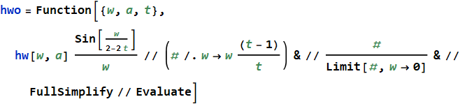
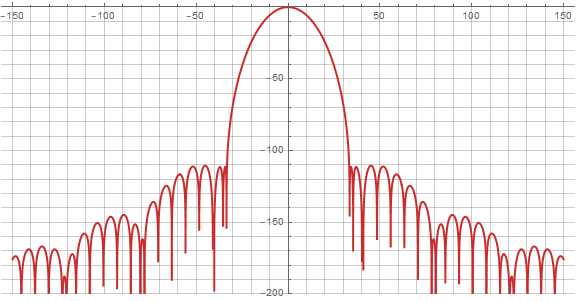
Now we can see how the spectrum changes in dynamics:







Here, changing the overlap parameter will already affect the window spectrum in a slightly different way :







Having played a little with the parameters, it is easy to notice that "more is not better", and the optimal degree of overlap for that function is in the region of four. Specifically, for t = 4 and a= 0.404 we get the side lobe level not exceeding -80 dB. This is a very good result - especially considering that the raised cosine function, traditionally used for summed windows, gives a lobe level of about -30 dB. Well, when written out explicitly, our new window function will look like this:

$$

$$\left\{ \begin{array}{ll} \frac{404 \pi (1-2 x)+36 \sin \left(\frac{1}{3} (16 \pi x+\pi )\right)+375 \sin \left(\frac{1}{3} (\pi -8 \pi x)\right)}{606 \pi } & \frac{1}{4} < x \leq \frac{1}{2} \\ \frac{404 (2 \pi x+\pi )+36 \sin \left(\frac{2}{3} \pi (8 x+1)\right)+375 \sin \left(\frac{1}{3} (8 \pi x+\pi )\right)}{606 \pi } & -\frac{1}{2} < x \leq -\frac{1}{4} \\ \frac{\sqrt{3} \left(125 \cos \left(\frac{8 \pi x}{3}\right)+12 \cos \left(\frac{16 \pi x}{3}\right)\right)}{202 \pi }+\frac{1}{3} & -\frac{1}{4} < x \leq \frac{1}{4} \\ 0 & \left| x\right| >\frac{1}{2} \\ \end{array} \right.$$

Further development

What else can you do to further reduce the sidelobe level? You can take cosines not with even, but with odd frequencies (here, for compactness, the solution of the system of equations is embedded directly into the definition of the function):

$$

$$\left(a \cos (\pi x)+\left(\frac{5}{8}-\frac{a}{2}\right) \cos (3 \pi x)+\left(\frac{3}{8}-\frac{a}{2}\right) \cos (5 \pi x)\right) \Pi (x)$$

and after integration with the parameters a = 0.6628 and an overlap level of 4.5, obtain an attenuation of -90 dB:







Explicitly:

$$

$$\small\left\{ \begin{array}{ll} \frac{327 \sin \left(\frac{1}{7} \pi (45 x+2)\right)+24855 \sin \left(\frac{1}{7} \pi (1-9 x)\right)+3670 \cos \left(\frac{1}{14} \pi (54 x+1)\right)+21512}{43024} & \frac{5}{18} < x \leq \frac{1}{2} \\ \frac{24855 \sin \left(\frac{1}{7} \pi (9 x+1)\right)+3670 \sin \left(\frac{3}{7} \pi (9 x+1)\right)+327 \sin \left(\frac{5}{7} \pi (9 x+1)\right)+21512}{43024} & -\frac{1}{2} < x \leq -\frac{5}{18} \\ \begin{array}{ll} \frac{-3670 \sin \left(\frac{3}{7} \pi (9 x-1)\right)+24855 \sin \left(\frac{1}{7} \pi (9 x+1)\right)+327 \sin \left(\frac{5}{7} \pi (9 x+1)\right)}{43024}+ \\ +\frac{3670 \sin \left(\frac{3}{7} \pi (9 x+1)\right)+327 \sin \left(\frac{1}{7} \pi (45 x+2)\right)+24855 \sin \left(\frac{1}{7} \pi (1-9 x)\right)}{43024} \end{array} & -\frac{5}{18} < x \leq \frac{5}{18} \\ 0 & \left| x\right| >\frac{1}{2} \\ \end{array} \right.$$

You can add one more cosine and increase the number of zero derivatives:

$$

$$\left(a \cos (\pi x)+\frac{1}{80} (35-16 a) \cos (3 \pi x)+\frac{1}{80} (35-48 a) \cos (5 \pi x)+\frac{1}{40} (5-8 a) \cos (7 \pi x)\right) \Pi (x)$$

and after integration with the parameters a = 0.5862 and the overlap level of 6.4, obtain a suppression of -110 dB:







Explicitly:

$$

$$\small\left\{ \begin{array}{ll} \frac{-3077550 \sin \left(\frac{1}{54} \pi (64 x-5)\right)-90069 \sin \left(\frac{5}{54} \pi (64 x-5)\right)-5820 \sin \left(\frac{7}{54} \pi (64 x-5)\right)-560455 \cos \left(\frac{1}{9} \pi (7-32 x)\right)+2601344}{5202688} & \frac{11}{32}< x \leq \frac{1}{2} \\ \frac{560455 \sin \left(\frac{1}{18} \pi (64 x+5)\right)+3077550 \sin \left(\frac{1}{54} \pi (64 x+5)\right)+90069 \sin \left(\frac{5}{54} \pi (64 x+5)\right)+5820 \sin \left(\frac{7}{54} \pi (64 x+5)\right)+2601344}{5202688} & -\frac{1}{2}< x \leq -\frac{11}{32} \\ \begin{array}{ll} \frac{-3077550 \sin \left(\frac{1}{54} \pi (64 x-5)\right)-90069 \sin \left(\frac{5}{54} \pi (64 x-5)\right)-5820 \sin \left(\frac{7}{54} \pi (64 x-5)\right)-560455 \cos \left(\frac{1}{9} \pi (7-32 x)\right)}{5202688}+ \\ +\frac{560455 \sin \left(\frac{1}{18} \pi (64 x+5)\right)+3077550 \sin \left(\frac{1}{54} \pi (64 x+5)\right)+90069 \sin \left(\frac{5}{54} \pi (64 x+5)\right)+5820 \sin \left(\frac{7}{54} \pi (64 x+5)\right)}{5202688} \end{array} &-\frac{11}{32}< x \leq \frac{11}{32} \\ 0 & \left| x\right| >\frac{1}{2} \\ \end{array} \right.$$

An even more significant reduction in the level of side lobes can be achieved by squaring the Fourier transform and thereby reducing the level of side lobes by a factor of 2 at once. This allows you to get rid of the increase in the number of parameters for their manual selection, but adds complexity in calculating the convolution in the time domain.









and here it is already possible to achieve suppression over 160 dB:







We will not give the formula explicitly because of its impressive size.

Hypergeometric window functions

To ensure the required number of zeros at the boundaries of our function, we used a search through the solution of a system of equations with subsequent integration. This is not very convenient - you have to change the number of equations every time. Maybe there is a simpler and more beautiful solution? There is! And the hypergeometric function will help us with this.





Our solution will look like this:

$$

$$\frac{2 z \Gamma \left(\frac{n+3}{2}\right) \, _2F_1\left(\frac{1}{2},-\frac{n}{2};\frac{3}{2};z^2\right)}{\sqrt{\pi } \Gamma \left(\frac{n}{2}+1\right)}+a \left(z+b z^3\right) \left(1-z^2\right)^{n/2}$$

Where $$$z=\sin \left(\frac{\pi x}{2}\right)$



It consists of the sum of two parts: the antiderivative of the function $$$\left(1-z^2\right)^{\frac{n}{2}}$normalized in amplitude to the point (1,1) and a function with free parameters, multiplied by the same $$$\left(1-z^2\right)^{\frac{n}{2}}$in order to preserve the required number of zero derivatives: The







accuracy of the adjustment and their influence on the distribution of side lobes will depend on which function we choose to correct the shape - there are possible options that require separate studies. In this case, the function$$$a \left(z+b z^3\right)$gives a completely acceptable option - and due to two parameters allows you to make more precise settings.



The formula itself is interesting (and convenient) in that for even n it is simplified to a polynomial, and for odd n it is simplified to the sum of a polynomial with arcsine and square root - which makes the final formula more compact and easier to calculate.



It is already easier (and faster) to select the parameters here through the discrete Fourier transform. We also need an additional definition of the overlap function to work with three parameters:



















As an example, after substituting the parameters from the picture, our function will be simplified to

$$

$$\frac{-288 z^{11}+2315 z^9-7380 z^7+12330 z^5-11940 z^3+8163 z}{3200}$$

Inverse Kaiser Window

If the task of summing the windows into one is not worth it, then the most optimal window is the Kaiser window, which allows you to smoothly adjust the width of the main lobe. However, it has a drawback - since it is expressed in terms of the Bessel function , it is somewhat difficult to read it outside the mathematical packages. You can, of course, separately implement the Bessel function - or you can look for an approximation through elementary functions. And suddenly it turned out that using the function of the spectrum of the Kaiser window (limited in time) for this, you can get even a little better result -

$$

$$\frac{ \sinh \left(k \sqrt{1-4 x^2}\right)}{\sinh (k) \sqrt{1-4 x^2} } \Pi (x)$$

The payment for such a cunning decision was the impossibility of expressing its spectrum purely analytically - but this is not so important, because in practice, in any case, we operate and analyze data in discrete form using the discrete Fourier transform. Below on the graph you can compare their spectra, where red is the original Kaiser window, green is its approximation:









With the same width of the main petal, the level of the side lobes is slightly lower. And for ease of use, you can draw up a table with approximate values ​​of the parameter k to obtain the required level of sidelobe suppression:

$$

$$\begin{array}{cc} \text{-60 } & \text{k=8.8} \\ \text{-90 } & \text{k=11.36} \\ \text{-120 } & \text{k=15.18} \\ \text{-150 } & \text{k=18.88} \\ \end{array}$$

Finding an approximation of the antiderivative of the inverse Kaiser window remains a separate interesting problem. So far, it has only been possible to express it through a power series, which converges rather slowly:

$$

$$\small \int \frac{ \sinh \left(k \sqrt{1-4 x^2}\right)}{\sinh (k) \sqrt{1-4 x^2} } \, dx= \sum _{n=1}^{\infty } -\frac{2^{\frac{1}{2}-n} k^{n-1} x^{2 n-1} \left(\sqrt{-k} (-1)^n K_{n-\frac{1}{2}}(-k)+\sqrt{k} K_{n-\frac{1}{2}}(k)\right)}{\sqrt{\pi } (2 n-1) \sinh (k) \Gamma (n)}$$

Perhaps experts in mathematics can suggest a better solution in the comments.

Conclusion

Despite the fact that digital signal processing is a completely formed discipline, there is still room for development and finding something new in it - at least in the existing special and scientific literature, the issues of constructing window functions summed up into a unit are not considered; and the capabilities of modern computer algebra systems allow rethinking the accumulated knowledge at a qualitatively new level.



The original Wolfram Mathematica document with all the calculations is available on GitHub .