
When I started my career as a developer, my first job was a DBA (database administrator, DBA). In those years, even before AWS RDS, Azure, Google Cloud and other cloud services, there were two types of DBAs:
- , . « », , .
- : , , SQL. ETL- . , .
Application DBAs have usually been part of development teams. They had deep knowledge of a specific topic, so they usually only worked on one or two projects. Infrastructure DBAs were usually part of the IT team and could work on multiple projects at the same time.
I am the application database admin
I never had the urge to mess around with backups or tweak storage (I'm sure it's fun!). To this day, I like to say that I'm a DB admin who knows how to develop applications, not a developer who understands databases.
In this article, I'll share some of the database development tricks I've learned over the course of my career.
Content:
- Update only what needs to be updated
- Disable constraints and indexes for heavy loads
- Use UNLOGGED tables for intermediate data
- Implement Entire Processes with WITH and RETURNING
- Avoid indices in columns with low selectivity
- Use partial indexes
- Always load sorted data
- Highly correlated columns index with BRIN
- Make indexes "invisible"
- Don't schedule long processes to start at the start of any hour
- Conclusion
Update only what needs to be updated
The operation
UPDATEconsumes quite a lot of resources. The best way to speed it up is to update only what needs to be updated.
Here's an example of a request to normalize an email column:
db=# UPDATE users SET email = lower(email);
UPDATE 1010000
Time: 1583.935 ms (00:01.584)
Looks innocent, right? The request updates mail addresses for 1,010,000 users. But do all the rows need to be updated?
db=# UPDATE users SET email = lower(email)
db-# WHERE email != lower(email);
UPDATE 10000
Time: 299.470 ms
Only 10,000 rows needed to be updated. By reducing the amount of data processed, we reduced the execution time from 1.5 seconds to less than 300ms. This will also save us further effort in maintaining the database.

Only update what needs to be updated.
This type of large update is very common in data migration scripts. The next time you write a script like this, make sure to update only what is needed.
Disable constraints and indexes for heavy loads
Constraints are an important part of relational databases: they preserve the consistency and reliability of the data. But everything has its own price, and more often than not, you have to pay when loading or updating a large number of rows.
Let's define a small storage schema:
DROP TABLE IF EXISTS product CASCADE;
CREATE TABLE product (
    id serial PRIMARY KEY,
    name TEXT NOT NULL,
    price INT NOT NULL
);
INSERT INTO product (name, price)
    SELECT random()::text, (random() * 1000)::int
    FROM generate_series(0, 10000);

DROP TABLE IF EXISTS customer CASCADE;
CREATE TABLE customer (
    id serial PRIMARY KEY,
    name TEXT NOT NULL
);
INSERT INTO customer (name)
    SELECT random()::text
    FROM generate_series(0, 100000);

DROP TABLE IF EXISTS sale;
CREATE TABLE sale (
    id serial PRIMARY KEY,
    created timestamptz NOT NULL,
    product_id int NOT NULL,
    customer_id int NOT NULL
);
It defines different types of constraints such as "not null" as well as unique constraints ...
To set the starting point, let's start adding
saleforeign keys to the table
db=# ALTER TABLE sale ADD CONSTRAINT sale_product_fk
db-# FOREIGN KEY (product_id) REFERENCES product(id);
ALTER TABLE
Time: 18.413 ms

db=# ALTER TABLE sale ADD CONSTRAINT sale_customer_fk
db-# FOREIGN KEY (customer_id) REFERENCES customer(id);
ALTER TABLE
Time: 5.464 ms

db=# CREATE INDEX sale_created_ix ON sale(created);
CREATE INDEX
Time: 12.605 ms

db=# INSERT INTO SALE (created, product_id, customer_id)
db-# SELECT
db-#    now() - interval '1 hour' * random() * 1000,
db-#    (random() * 10000)::int + 1,
db-#    (random() * 100000)::int + 1
db-# FROM generate_series(1, 1000000);
INSERT 0 1000000
Time: 15410.234 ms (00:15.410)
After defining the constraints and indexes, loading a million rows into the table took about 15.4 seconds.
Now, first, let's load the data into the table, and only then add constraints and indexes:
db=# INSERT INTO SALE (created, product_id, customer_id)
db-# SELECT
db-#    now() - interval '1 hour' * random() * 1000,
db-#    (random() * 10000)::int + 1,
db-#    (random() * 100000)::int + 1
db-# FROM generate_series(1, 1000000);
INSERT 0 1000000
Time: 2277.824 ms (00:02.278)

db=# ALTER TABLE sale ADD CONSTRAINT sale_product_fk
db-# FOREIGN KEY (product_id) REFERENCES product(id);
ALTER TABLE
Time: 169.193 ms

db=# ALTER TABLE sale ADD CONSTRAINT sale_customer_fk
db-# FOREIGN KEY (customer_id) REFERENCES customer(id);
ALTER TABLE
Time: 185.633 ms

db=# CREATE INDEX sale_created_ix ON sale(created);
CREATE INDEX
Time: 484.244 ms
Loading was much faster, 2.27 seconds. instead of 15.4. Indexes and limits were created much longer after loading the data, but the whole process was much faster: 3.1 seconds. instead of 15.4.
Unfortunately, in PostgreSQL you cannot do the same with indexes, you can only throw them away and recreate them. In other databases, such as Oracle, you can disable and enable indexes without rebuilding.
UNLOGGED-
When you change data in PostgreSQL, the changes are written to the write ahead log (WAL ). It is used to maintain consistency, quickly reindex during recovery, and maintain replication.
Writing to WAL is often needed, but there are some circumstances in which you can opt out of WAL to speed things up. For example, in the case of intermediate tables.
Intermediate tables are called one-off tables, which store temporary data used to implement some processes. For example, in ETL processes, it is very common to load data from CSV files into staging tables, clear the information, and then load it into the target table. In this scenario, the staging table is one-time use and is not used in backups or replicas.

UNLOGGED table.
Staging tables that do not need to be recovered in the event of a failure and are not needed in replicas can be set as UNLOGGED :
CREATE UNLOGGED TABLE staging_table ( /* table definition */ );
Caution : Before using
UNLOGGED, make sure you fully understand all the implications.
Implement Entire Processes with WITH and RETURNING
Let's say you have a users table and you find that it contains duplicate data:
Table setup
db=# SELECT u.id, u.email, o.id as order_id
FROM orders o JOIN users u ON o.user_id = u.id;

 id |       email       | order_id
----+-------------------+----------
  1 | foo@bar.baz       |        1
  1 | foo@bar.baz       |        2
  2 | me@hakibenita.com |        3
  3 | ME@hakibenita.com |        4
  3 | ME@hakibenita.com |        5
User haki benita registered twice, with mail
ME@hakibenita.comand me@hakibenita.com. Since we are not normalizing email addresses when entering them into the table, now we have to deal with duplicates.
We need:
- Identify duplicate addresses in lowercase letters and link duplicate users to each other.
- Update orders so that they only refer to one of the duplicates.
- Remove duplicates from the table.
You can link duplicate users using a staging table:
db=# CREATE UNLOGGED TABLE duplicate_users AS
db-#     SELECT
db-#         lower(email) AS normalized_email,
db-#         min(id) AS convert_to_user,
db-#         array_remove(ARRAY_AGG(id), min(id)) as convert_from_users
db-#     FROM
db-#         users
db-#     GROUP BY
db-#         normalized_email
db-#     HAVING
db-#         count(*) > 1;
CREATE TABLE

db=# SELECT * FROM duplicate_users;
 normalized_email  | convert_to_user | convert_from_users
-------------------+-----------------+--------------------
 me@hakibenita.com |               2 | {3}
The intermediate table contains links between takes. If a user with a normalized email address appears more than once, we assign him a minimum user ID, into which we collapse all duplicates. The rest of the users are stored in the array column and all links to them will be updated.
Using the intermediate table, we will update the links to duplicates in the table
orders:
db=# UPDATE
db-#    orders o
db-# SET
db-#    user_id = du.convert_to_user
db-# FROM
db-#    duplicate_users du
db-# WHERE
db-#    o.user_id = ANY(du.convert_from_users);
UPDATE 2
Now you can safely remove duplicates from
users:
db=# DELETE FROM
db-#    users
db-# WHERE
db-#    id IN (
db(#        SELECT unnest(convert_from_users)
db(#        FROM duplicate_users
db(#    );
DELETE 1
Note that we used the unnest function to "transform" the array , which turns each element into a string.
Result:
db=# SELECT u.id, u.email, o.id as order_id
db-# FROM orders o JOIN users u ON o.user_id = u.id;
 id |       email       | order_id
----+-------------------+----------
  1 | foo@bar.baz       |        1
  1 | foo@bar.baz       |        2
  2 | me@hakibenita.com |        3
  2 | me@hakibenita.com |        4
  2 | me@hakibenita.com |        5
Great, all user
3( ME@hakibenita.com) instances are converted to user 2( me@hakibenita.com).
We can also check that duplicates are removed from the table
users:
db=# SELECT * FROM users;
 id |       email
----+-------------------
  1 | foo@bar.baz
  2 | me@hakibenita.com
Now you can get rid of the staging table:
db=# DROP TABLE duplicate_users;
DROP TABLE
All is well, but too long and needs cleaning! Is there a better way?
Generalized Table Expressions (CTE)
With generic table expressions , also known as expressions
WITH, we can execute the entire procedure with a single SQL expression:
WITH duplicate_users AS (
    SELECT
        min(id) AS convert_to_user,
        array_remove(ARRAY_AGG(id), min(id)) as convert_from_users
    FROM
        users
    GROUP BY
        lower(email)
    HAVING
        count(*) > 1
),

update_orders_of_duplicate_users AS (
    UPDATE
        orders o
    SET
        user_id = du.convert_to_user
    FROM
        duplicate_users du
    WHERE
        o.user_id = ANY(du.convert_from_users)
)

DELETE FROM
    users
WHERE
    id IN (
        SELECT
            unnest(convert_from_users)
        FROM
            duplicate_users
    );
Instead of a staging table, we created a generic table expression and reused it.
Returning results from CTE
One of the advantages of executing DML within an expression
WITHis that you can return data from it using the RETURNING keyword . Let's say we need a report on the number of updated and deleted rows:
WITH duplicate_users AS (
    SELECT
        min(id) AS convert_to_user,
        array_remove(ARRAY_AGG(id), min(id)) as convert_from_users
    FROM
        users
    GROUP BY
        lower(email)
    HAVING
        count(*) > 1
),

update_orders_of_duplicate_users AS (
    UPDATE
        orders o
    SET
        user_id = du.convert_to_user
    FROM
        duplicate_users du
    WHERE
        o.user_id = ANY(du.convert_from_users)
    RETURNING o.id
),

delete_duplicate_user AS (
    DELETE FROM
        users
    WHERE
        id IN (
            SELECT unnest(convert_from_users)
            FROM duplicate_users
        )
        RETURNING id
)

SELECT
    (SELECT count(*) FROM update_orders_of_duplicate_users) AS orders_updated,
    (SELECT count(*) FROM delete_duplicate_user) AS users_deleted
;
Result:
orders_updated | users_deleted
----------------+---------------
              2 |             1
The beauty of this approach is that the entire process is done with a single command, so there is no need to manage transactions or worry about flushing the staging table if the process crashes.
Warning : A Reddit reader pointed out to me the possible unpredictable behavior of DML execution in generic table expressions :
The subexpressions inWITHare executed concurrently with each other and with the main query. Therefore, when used inWITHdata-modifying expressions, the actual order of updates will be unpredictable.
This means that you cannot rely on the order in which independent subexpressions are executed. It turns out that if there is a dependency between them, as in the example above, you can rely on the execution of the dependent subexpression before using them.
Avoid indices in columns with low selectivity
Let's say you have a signup process where a user logs in at an email address. To activate your account, you need to verify your mail. The table might look like this:
db=# CREATE TABLE users (
db-#    id serial,
db-#    username text,
db-#    activated boolean
db-#);
CREATE TABLE
Most of your users are citizens conscious, they register with the correct mailing address and immediately activate the account. Let's fill the table with user data, and assume that 90% of users are activated:
db=# INSERT INTO users (username, activated)
db-# SELECT
db-#     md5(random()::text) AS username,
db-#     random() < 0.9 AS activated
db-# FROM
db-#     generate_series(1, 1000000);
INSERT 0 1000000

db=# SELECT activated, count(*) FROM users GROUP BY activated;
 activated | count
-----------+--------
 f         | 102567
 t         | 897433

db=# VACUUM ANALYZE users;
VACUUM
To query the number of activated and non-activated users, you can create an index by column
activated:
db=# CREATE INDEX users_activated_ix ON users(activated);
CREATE INDEX
And if you ask for the number of non-activated users , the database will use the index:
db=# EXPLAIN SELECT * FROM users WHERE NOT activated;
                                      QUERY PLAN
--------------------------------------------------------------------------------------
 Bitmap Heap Scan on users  (cost=1923.32..11282.99 rows=102567 width=38)
   Filter: (NOT activated)
   ->  Bitmap Index Scan on users_activated_ix  (cost=0.00..1897.68 rows=102567 width=0)
         Index Cond: (activated = false)
The base decided that the filter would return 102,567 items, roughly 10% of the table. This is consistent with the data we loaded, so the table did a good job.
However, if we query the number of activated users , we find that the database has decided not to use the index :
db=# EXPLAIN SELECT * FROM users WHERE activated;
                          QUERY PLAN
---------------------------------------------------------------
 Seq Scan on users  (cost=0.00..18334.00 rows=897433 width=38)
   Filter: activated
Many developers are confused when the database is not using the index. To explain why it does this, the following is: if you needed to read the entire table, would you use an index ?
Probably not, why is this necessary? Reading from disk is expensive, so you'll want to read as little as possible. For example, if the table is 10 MB and the index is 1 MB, then to read the entire table, you will have to read 10 MB from disk. And if you add an index, you get 11 MB. It's wasteful.
Let's now take a look at the statistics that PostgreSQL has collected on our table:
db=# SELECT attname, n_distinct, most_common_vals, most_common_freqs
db-# FROM pg_stats
db-# WHERE tablename = 'users' AND attname='activated';
------------------+------------------------
attname           | activated
n_distinct        | 2
most_common_vals  | {t,f}
most_common_freqs | {0.89743334,0.10256667}
When PostgreSQL parsed the table, it found that
activatedthere were two different values in the column . The value tin the column most_common_valscorresponds to the frequency 0.89743334in the column most_common_freqs, and the value fcorresponds to the frequency 0.10256667. After analyzing the table, the database determined that 89.74% of the records were activated users and the remaining 10.26% were non-activated.
Based on these statistics, PostgreSQL decided that it is better to scan the entire table than to assume that 90% of the rows satisfy the condition. The threshold beyond which a base can decide whether to use an index depends on many factors, and there is no rule of thumb.
Index for columns with low and high selectivity.
Use partial indexes
In the previous chapter, we created an index for a boolean column that had about 90% of the records
true(activated users).
When we asked for the number of active users, the database did not use the index. And when asked for the number of non-activated, the database used the index.
The question arises: if the database is not going to use the index to filter out active users, why would we index them in the first place?
Before answering this question, let's look at the weight of the full index by column
activated:
db=# \di+ users_activated_ix

 Schema |      Name          | Type  | Owner | Table | Size
--------+--------------------+-------+-------+-------+------
 public | users_activated_ix | index | haki  | users | 21 MB
The index weighs 21 MB. Just for reference: the table with users is 65 MB. That is, the index weight is ~ 32% of the base weight. That being said, we know that ~ 90% of the index content is unlikely to be used.
In PostgreSQL, you can create an index on only a portion of a table - the so-called partial index :
db=# CREATE INDEX users_unactivated_partial_ix ON users(id)
db-# WHERE not activated;
CREATE INDEX
We use an expression
WHEREto constrain the strings covered by the index. Let's check if it works:
db=# EXPLAIN SELECT * FROM users WHERE not activated;
                                           QUERY PLAN
------------------------------------------------------------------------------------------------
 Index Scan using users_unactivated_partial_ix on users  (cost=0.29..3493.60 rows=102567 width=38)
Great, the database turned out to be smart enough to realize that the Boolean expression we used in our query might work for a partial index.
This approach has another advantage:
db=# \di+ users_unactivated_partial_ix
                                 List of relations
 Schema |           Name               | Type  | Owner | Table |  Size
--------+------------------------------+-------+-------+-------+---------
 public | users_unactivated_partial_ix | index | haki  | users | 2216 kB
The full column index weighs 21 MB, and the partial index is only 2.2 MB. That is 10%, which corresponds to the proportion of non-activated users in the table.
Always load sorted data
This is one of my most frequent comments when parsing code. The advice is not as intuitive as the others and can have a huge impact on productivity.
Let's say you have a huge table with specific sales:
db=# CREATE TABLE sale_fact (id serial, username text, sold_at date);
CREATE TABLE
Every night during the ETL process, you load data into a table:
db=# INSERT INTO sale_fact (username, sold_at)
db-# SELECT
db-#     md5(random()::text) AS username,
db-#     '2020-01-01'::date + (interval '1 day') * round(random() * 365 * 2) AS sold_at
db-# FROM
db-#     generate_series(1, 100000);
INSERT 0 100000

db=# VACUUM ANALYZE sale_fact;
VACUUM
To simulate the download, we use random data. We inserted 100 thousand lines with random names, and the sales dates for the period from January 1, 2020 and two years ahead.
For the most part, the table is used for summary sales reports. Most often, they filter by date to see sales for a specific period. To speed up the range scan, let's create an index by
sold_at:
db=# CREATE INDEX sale_fact_sold_at_ix ON sale_fact(sold_at);
CREATE INDEX
Let's take a look at the execution plan for the request to fetch all sales in June 2020:
db=# EXPLAIN (ANALYZE)
db-# SELECT *
db-# FROM sale_fact
db-# WHERE sold_at BETWEEN '2020-07-01' AND '2020-07-31';

                            QUERY PLAN
-----------------------------------------------------------------------------------------------
 Bitmap Heap Scan on sale_fact  (cost=108.30..1107.69 rows=4293 width=41)
   Recheck Cond: ((sold_at >= '2020-07-01'::date) AND (sold_at <= '2020-07-31'::date))
   Heap Blocks: exact=927
   ->  Bitmap Index Scan on sale_fact_sold_at_ix  (cost=0.00..107.22 rows=4293 width=0)
         Index Cond: ((sold_at >= '2020-07-01'::date) AND (sold_at <= '2020-07-31'::date))
 Planning Time: 0.191 ms
 Execution Time: 5.906 ms
After running the request several times to warm up the cache, the execution time stabilized at the level of 6 ms.
Bitmap Scan
In terms of execution, we see that the base used bitmap scanning. It takes place in two stages:
(Bitmap Index Scan): the base goes through the entire indexsale_fact_sold_at_ixand finds all the pages in the table that contain the relevant rows.(Bitmap Heap Scan): the base reads the pages containing the relevant strings and finds those that satisfy the condition.
Pages can contain many lines. In the first step, the index is used to find pages . The second stage searches for lines in pages, hence the operation
Recheck Condin the execution plan follows .
At this point, many DBAs and developers will round off and move on to the next query. But there is a way to improve this query.
Index Scan
Let's make a small change to data loading.
db=# TRUNCATE sale_fact;
TRUNCATE TABLE

db=# INSERT INTO sale_fact (username, sold_at)
db-# SELECT
db-#     md5(random()::text) AS username,
db-#     '2020-01-01'::date + (interval '1 day') * round(random() * 365 * 2) AS sold_at
db-# FROM
db-#     generate_series(1, 100000)
db-# ORDER BY sold_at;
INSERT 0 100000

db=# VACUUM ANALYZE sale_fact;
VACUUM
This time we loaded data sorted by
sold_at.
Now the execution plan for the same query looks like this:
db=# EXPLAIN (ANALYZE)
db-# SELECT *
db-# FROM sale_fact
db-# WHERE sold_at BETWEEN '2020-07-01' AND '2020-07-31';

                           QUERY PLAN
---------------------------------------------------------------------------------------------
 Index Scan using sale_fact_sold_at_ix on sale_fact (cost=0.29..184.73 rows=4272 width=41)
   Index Cond: ((sold_at >= '2020-07-01'::date) AND (sold_at <= '2020-07-31'::date))
 Planning Time: 0.145 ms
 Execution Time: 2.294 ms
After several runs, the execution time stabilized at 2.3ms. We have achieved sustainable savings of around 60%.
We also see that this time the database did not use bitmap scanning, but applied a "normal" index scan. Why?
Correlation
When the database analyzes the table, it collects all the statistics it can get. One of the parameters is correlation :
Statistical correlation between the physical order of rows and the logical order of values in columns. If the value is around -1 or +1, an index scan across the column is considered more advantageous than when the correlation value is around 0, since the number of random disk accesses is reduced.
As explained in the official documentation, correlation is a measure of how the values in a particular column on disk are “sorted”.
Correlation = 1.
If the correlation is 1 or so, it means the pages are stored on disk in roughly the same order as the rows in the table. This is very common. For example, auto-incrementing IDs tend to have a correlation close to 1. Date and timestamp columns that show when the rows were created also have a correlation close to 1.
If the correlation is -1, the pages are sorted in reverse order of the columns.
Correlation ~ 0.
If the correlation is close to 0, it means that the values in the column do not correlate or hardly correlate with the page order in the table.
Let's go back to
sale_fact. When we loaded the data into the table without pre-sorting, the correlations were like this:
db=# SELECT tablename, attname, correlation
db-# FROM pg_stats
db=# WHERE tablename = 'sale_fact';

 tablename | attname  | correlation
-----------+----------+--------------
 sale      | id       |            1
 sale      | username | -0.005344716
 sale      | sold_at  | -0.011389783
The automatically generated column ID has a correlation of 1. The column has a
sold_atvery low correlation: consecutive values are scattered throughout the table.
When we loaded the sorted data into the table, she calculated the correlations:
tablename | attname  |  correlation
-----------+----------+----------------
 sale_fact | id       |              1
 sale_fact | username | -0.00041992788
 sale_fact | sold_at  |              1
The correlation
sold_atis now equal 1.
So why did the database use bitmap scans when the correlation was low, but index scans when the correlation was high?
- When the correlation was 1, the base determined that the rows of the requested range were likely to be in consecutive pages. Then it is better to use an index scan to read multiple pages.
- When the correlation was close to 0, the base determined that the rows of the requested range were likely to be scattered throughout the table. Then it is advisable to use a bitmap scan of those pages that contain the required lines, and only then extract them using the condition.
The next time you load data into a table, think about how much information will be requested and sort so that the indexes can quickly scan ranges.
CLUSTER Command
Another way to "sort a table on disk" by a specific index is to use the CLUSTER command .
For instance:
db=# TRUNCATE sale_fact;
TRUNCATE TABLE

-- Insert rows without sorting
db=# INSERT INTO sale_fact (username, sold_at)
db-# SELECT
db-#     md5(random()::text) AS username,
db-#     '2020-01-01'::date + (interval '1 day') * round(random() * 365 * 2) AS sold_at
db-# FROM
db-#     generate_series(1, 100000)
INSERT 0 100000

db=# ANALYZE sale_fact;
ANALYZE

db=# SELECT tablename, attname, correlation
db-# FROM pg_stats
db-# WHERE tablename = 'sale_fact';

  tablename | attname  |  correlation
-----------+-----------+----------------
 sale_fact | sold_at   | -5.9702674e-05
 sale_fact | id        |              1
 sale_fact | username  |    0.010033822
We loaded the data into the table in a random order, so the correlation
sold_atis close to zero.
To "recompose" the table by
sold_at, we use the command CLUSTERto sort the table on disk according to the index sale_fact_sold_at_ix:
db=# CLUSTER sale_fact USING sale_fact_sold_at_ix;
CLUSTER

db=# ANALYZE sale_fact;
ANALYZE

db=# SELECT tablename, attname, correlation
db-# FROM pg_stats
db-# WHERE tablename = 'sale_fact';

 tablename | attname  | correlation
-----------+----------+--------------
 sale_fact | sold_at  |            1
 sale_fact | id       | -0.002239401
 sale_fact | username |  0.013389298
After clustering the table, the correlation
sold_atbecame 1.
CLUSTER command.
Points to note:
- Clustering a table on a particular column can affect the correlation of another column. For example, take a look at the correlation of IDs after clustering by
sold_at. CLUSTERIs a heavy and blocking operation, so do not apply it to a live table.
For these reasons, it is best to insert data that is already sorted and not rely on
CLUSTER.
Highly correlated columns index with BRIN
When it comes to indexes, many developers think of B-trees. But PostgreSQL offers other types of indexes, such as BRIN :
BRIN is designed to work with very large tables in which some columns naturally correlate with their physical location within the table
BRIN stands for Block Range Index. According to the documentation, BRIN works best with highly correlated columns. As we have seen in previous chapters, auto-incrementing IDs and timestamps naturally correlate with the physical structure of the table, so BRIN is more beneficial for them.
Under certain conditions BRIN can provide better "value for money" in terms of size and performance compared to a comparable B-tree index.

BRIN.
BRIN is a range of values within several adjacent pages in a table. Let's say we have the following values in a column, each on a separate page:
1, 2, 3, 4, 5, 6, 7, 8, 9
BRIN works with ranges of adjacent pages. If you specify three adjacent pages, the index splits the table into ranges:
[1,2,3], [4,5,6], [7,8,9]
For each range, BRIN stores the minimum and maximum value :
[1–3], [4–6], [7–9]
Let's use this index to look for the value 5:
- [1–3] - he certainly isn't here.
- [4–6] - may be here.
- [7–9] - he certainly isn't here.
With BRIN we have limited the search area to block 4-6.
Let's take another example. Let the values in the column have a correlation close to zero, that is, they are not sorted:
[2,9,5], [1,4,7], [3,8,6]
Indexing three adjacent blocks will give us the following ranges:
[2–9], [1–7], [3–8]
Let's look for the value 5:
- [2-9] - may be here.
- [1-7] - may be here.
- [3–8] - may be here.
In this case, the index does not narrow the search at all, so it is useless.
Understanding pages_per_range
The number of adjacent pages is determined by the parameter
pages_per_range. The number of pages in a range affects the size and precision of the BRIN:
- A
pages_per_rangesmaller and less accurate index will give a big value . - A small value
pages_per_rangewill give a larger and more accurate index.
The default
pages_per_rangeis 128.

BRIN with lower pages_per_range.
To illustrate, let's create a BRIN with ranges of two pages and look for a value of 5:
- [1–2] - he certainly isn't here.
- [3–4] - he certainly isn't here.
- [5-6] - may be here.
- [7–8] - he certainly isn't here.
- [9] - it is definitely not here.
With a two-page range, we can restrict the search to blocks 5 and 6. If the range is three-page, the index will limit the search to blocks 4, 5, and 6.
Another difference between the two indexes is that when the range was three pages, we needed to store three ranges , and with two pages in a range, we already get five ranges and the index increases.
Create BRIN
Let's take a table
sales_factand create a BRIN by column sold_at:
db=# CREATE INDEX sale_fact_sold_at_bix ON sale_fact
db-# USING BRIN(sold_at) WITH (pages_per_range = 128);
CREATE INDEX
The default is
pages_per_range = 128.
Now let's query the sales date period:
db=# EXPLAIN (ANALYZE)
db-# SELECT *
db-# FROM sale_fact
db-# WHERE sold_at BETWEEN '2020-07-01' AND '2020-07-31';
                                    QUERY PLAN
--------------------------------------------------------------------------------------------
 Bitmap Heap Scan on sale_fact  (cost=13.11..1135.61 rows=4319 width=41)
   Recheck Cond: ((sold_at >= '2020-07-01'::date) AND (sold_at <= '2020-07-31'::date))
   Rows Removed by Index Recheck: 23130
   Heap Blocks: lossy=256
   ->  Bitmap Index Scan on sale_fact_sold_at_bix  (cost=0.00..12.03 rows=12500 width=0)
         Index Cond: ((sold_at >= '2020-07-01'::date) AND (sold_at <= '2020-07-31'::date))
 Execution Time: 8.877 ms
The base got the date period using BRIN, but this is nothing interesting ...
Optimizing pages_per_range
According to the execution plan, the database removed 23,130 rows from the pages, which it found using the index. This may indicate that the range we specified for the index is too large for this query. Let's create an index with half the number of pages in the range:
db=# CREATE INDEX sale_fact_sold_at_bix64 ON sale_fact
db-# USING BRIN(sold_at) WITH (pages_per_range = 64);
CREATE INDEX

db=# EXPLAIN (ANALYZE)
db- SELECT *
db- FROM sale_fact
db- WHERE sold_at BETWEEN '2020-07-01' AND '2020-07-31';
                                        QUERY PLAN
---------------------------------------------------------------------------------------------
 Bitmap Heap Scan on sale_fact  (cost=13.10..1048.10 rows=4319 width=41)
   Recheck Cond: ((sold_at >= '2020-07-01'::date) AND (sold_at <= '2020-07-31'::date))
   Rows Removed by Index Recheck: 9434
   Heap Blocks: lossy=128
   ->  Bitmap Index Scan on sale_fact_sold_at_bix64  (cost=0.00..12.02 rows=6667 width=0)
         Index Cond: ((sold_at >= '2020-07-01'::date) AND (sold_at <= '2020-07-31'::date))
 Execution Time: 5.491 ms
With 64 pages in the range, the base deleted fewer rows found using the index - 9 434. This means it had to do fewer I / O operations, and the query was executed a little faster, in ~ 5.5 ms instead of ~ 8.9.
Let's test the index with different values
pages_per_range:
| pages_per_range | Removed rows when re-checking index |
| 128 | 23130 |
| 64 | 9 434 |
| 8 | 874 |
| 4 | 446 |
| 2 | 446 |
Decreasing the
pages_per_rangeindex becomes more precise, and it removes fewer rows from the pages it finds.
Please note that we have optimized a very specific query. This is fine for illustration, but in real life it is better to use values that meet the needs of most queries.
Estimating the size of the index
Another major advantage of BRIN is its size. In previous chapters, we
sold_atcreated a B-tree index for a field . Its size was 2,224 KB. And the BRIN size with the parameter is pages_per_range=128only 48 KB: 46 times smaller.
Schema |         Name          | Type  | Owner |   Table   | Size
--------+-----------------------+-------+-------+-----------+-------
 public | sale_fact_sold_at_bix | index | haki  | sale_fact | 48 kB
 public | sale_fact_sold_at_ix  | index | haki  | sale_fact | 2224 kB
BRIN size is also affected
pages_per_range. For example, BRIN s pages_per_range=2weighs 56 Kb, slightly more than 48 Kb.
Make indexes "invisible"
PostgreSQL has a cool transactional DDL feature . Over the years with Oracle, I have grown accustomed to using DDL commands such as
CREATE, DROPand at the end of transactions ALTER. But in PostgreSQL, you can execute DDL commands inside a transaction, and changes will be applied only after the transaction is committed.
I recently discovered that using transactional DDL can make indexes invisible! This is useful when you want to see an execution plan without indexes.
For example, in a table
sale_factwe have created an index on a column sold_at. The execution plan for the July sales fetch request looks like this:
db=# EXPLAIN
db-# SELECT *
db-# FROM sale_fact
db-# WHERE sold_at BETWEEN '2020-07-01' AND '2020-07-31';
                                         QUERY PLAN
--------------------------------------------------------------------------------------------
 Index Scan using sale_fact_sold_at_ix on sale_fact  (cost=0.42..182.80 rows=4319 width=41)
   Index Cond: ((sold_at >= '2020-07-01'::date) AND (sold_at <= '2020-07-31'::date))P
To see what the plan would look like if there were no index
sale_fact_sold_at_ix, you can put the index inside a transaction and roll back immediately:
db=# BEGIN;
BEGIN

db=# DROP INDEX sale_fact_sold_at_ix;
DROP INDEX

db=# EXPLAIN
db-# SELECT *
db-# FROM sale_fact
db-# WHERE sold_at BETWEEN '2020-07-01' AND '2020-07-31';
                                   QUERY PLAN
---------------------------------------------------------------------------------

 Seq Scan on sale_fact  (cost=0.00..2435.00 rows=4319 width=41)
   Filter: ((sold_at >= '2020-07-01'::date) AND (sold_at <= '2020-07-31'::date))

db=# ROLLBACK;
ROLLBACK
First, let's start a transaction with
BEGIN. Then we drop the index and generate the execution plan. Note that the plan now uses a full table scan as if the index did not exist. At this point, the transaction is still in progress, so the index has not been dropped yet. To complete the transaction without dropping the index, roll it back using the command ROLLBACK.
Let's check that the index still exists:
db=# \di+ sale_fact_sold_at_ix
                                 List of relations
 Schema |         Name         | Type  | Owner |   Table   |  Size
--------+----------------------+-------+-------+-----------+---------
 public | sale_fact_sold_at_ix | index | haki  | sale_fact | 2224 kB
Other databases that do not support transactional DDL may accomplish the goal differently. For example, Oracle allows you to mark an index as invisible and the optimizer will then ignore it.
Warning : if you to drop the index inside a transaction, it will lead to the blocking of competitive operations
SELECT, INSERT, UPDATEand DELETEin the table until the transaction is active. Use with caution in test environments and avoid use in production facilities.
Don't schedule long processes to start at the start of any hour
Investors know that strange things can happen when the stock price reaches beautiful round values, for example, $ 10, $ 100, $ 1000. Here's what they write about it :
[...] the price of assets can change unpredictably, crossing round values like $ 50 or $ 100 per share. Many inexperienced traders like to buy or sell assets when the price reaches round numbers because they think they are fair prices.
From this point of view, developers are not very different from investors. When they need to schedule a long process, they usually choose an hour.
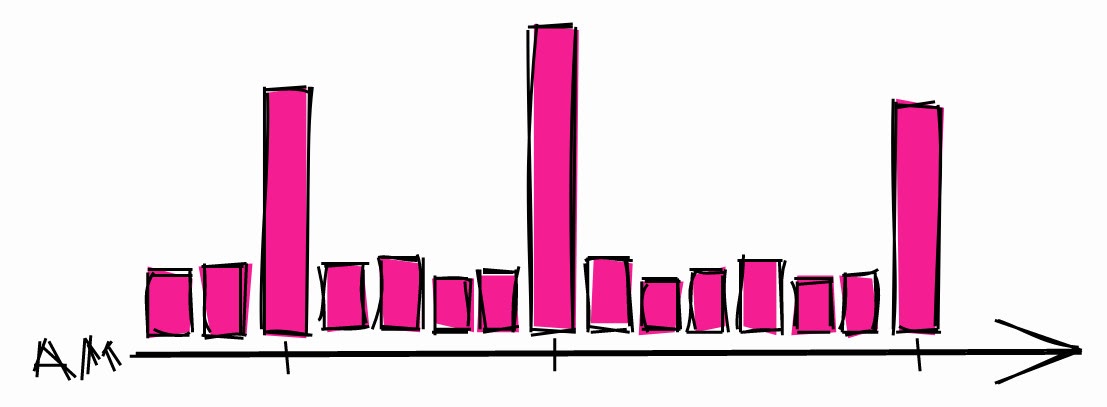
Typical overnight system load.
This can lead to spikes in load during these hours. So if you need to schedule a long process, there is a greater chance that the system will be idle at other times.
It is also recommended to use random delays in the schedules so as not to start at the same time every time. Then even if another task is scheduled for this hour, it will not be a big problem. If you are using a systemd timer, you can use the RandomizedDelaySec option .
Conclusion
This article provides tips of varying degrees of evidence based on my experience. Some are easy to implement, some require a deep understanding of how databases work. Databases are the backbone of most modern systems, so the time spent learning how to work is a good investment for any developer!