
Source: Vecteezy
Yes, linear regression is not the only one.
Quickly name five machine learning algorithms.
It is unlikely that you will name many regression algorithms. After all, the only widely used regression algorithm is linear regression, mainly because of its simplicity. However, linear regression is often inapplicable to real data due to too limited options and limited freedom of maneuver. It is often used only as a baseline model for evaluation and comparison with new research approaches. Mail.ru Cloud Solutions
teamtranslated an article, the author of which describes 5 regression algorithms. They are worth having in your toolbox along with popular classification algorithms such as SVM, decision tree and neural networks.
1. Neural network regression
Theory
Neural networks are incredibly powerful, but they are commonly used for classification. Signals travel through layers of neurons and are generalized into one of several classes. However, they can be very quickly adapted into regression models by changing the last activation function.
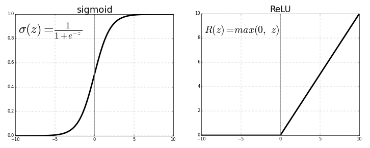
Each neuron transmits values from the previous connection through an activation function serving the purpose of generalization and non-linearity. Usually the activation function is something like a sigmoid or a ReLU (rectified linear unit) function.
Source . Free image
But, replacing the last activation function (output neuron) with a linear onethe activation function, the output signal can be mapped to many values outside the fixed classes. Thus, the output will not be the probability of assigning the input signal to any one class, but a continuous value at which the neural network fixes its observations. In this sense, we can say that the neural network complements linear regression.
Neural network regression has the advantage of non-linearity (in addition to complexity) that can be introduced with sigmoid and other non-linear activation functions earlier in the neural network. However, overuse of ReLU as an activation function may mean that the model tends to avoid outputting negative values, since ReLU ignores the relative differences between negative values.
This can be solved either by limiting the use of ReLU and adding more negative values of the corresponding activation functions, or by normalizing the data to a strictly positive range before training.
Implementation
Using Keras, let's build the structure of an artificial neural network, although the same could be done with a convolutional neural network or another network if the last layer is either a dense layer with linear activation or just a layer with linear activation. ( Note that Keras imports are not listed to save space ).
model = Sequential()
model.add(Dense(100, input_dim=3, activation='sigmoid'))
model.add(ReLU(alpha=1.0))
model.add(Dense(50, activation='sigmoid'))
model.add(ReLU(alpha=1.0))
model.add(Dense(25, activation='softmax'))
#IMPORTANT PART
model.add(Dense(1, activation='linear'))
The problem with neural networks has always been their high variance and tendency to overfit. There are many sources of non-linearity in the above code example like SoftMax or sigmoid.
If your neural network does a good job with training data with a purely linear structure, it might be better to use truncated decision tree regression, which emulates a linear and highly dispersed neural network, but allows the data scientist to have better control over depth, width, and other attributes to control overfitting.
2. Decision tree regression
Theory
Decision trees in classification and regression are very similar in that they work by constructing trees with yes / no nodes. However, while classification leaf nodes result in a single class value (for example, 1 or 0 for a binary classification problem), regression trees end up with a value in continuous mode (for example, 4593.49 or 10.98).
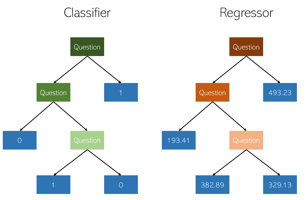
Illustration by the author
Due to the specific and highly dispersed nature of regression as a mere machine learning problem, decision tree regressors should be carefully pruned. However, the regression approach is irregular - instead of calculating the value on a continuous scale, it arrives at given end nodes. If the regressor is clipped too much, it has too few leaf nodes to properly fulfill its purpose.
Consequently, the decision tree should be pruned so that it has the most freedom (the possible output values of the regression are the number of leaf nodes), but not enough to be too deep. If you don't cut it off, the already highly dispersed algorithm will become overly complex due to the nature of the regression.
Implementation
Decision tree regression can be easily created in
sklearn:
from sklearn.tree import DecisionTreeRegressor
model = DecisionTreeRegressor()
model.fit(X_train, y_train)
Since the parameters of the decision tree regressor very important, it is recommended to use a search engine optimization tool parameters
GridCVfrom sklearn, to find the right recommendation for this model.
When evaluating performance formally, use testing
K-foldinstead of standard testing train-test-splitto avoid the latter's randomness that might violate the sensitive results of the high variance model.
Bonus: A close relative of the decision tree, the random forest algorithm, can also be implemented as a regressor. A random forest regressor may or may not perform better than a decision tree in regression (while it usually performs better in classification) due to the delicate balance between redundancy and inadequacy in tree building algorithms.
from sklearn.ensemble import RandomForestRegressor
model = RandomForestRegressor()
model.fit(X_train, y_train)
3. LASSO regression
The lasso regression method (LASSO, Least Absolute Shrinkage and Selection Operator) is a variation of linear regression specially adapted for data that exhibits strong multicollinearity (that is, strong correlation of features with each other).
It automates parts of model selection, such as variable selection or parameter exclusion. LASSO uses shrinkage, which is a process in which data values approach a center point (such as an average).

Author's illustration. Simplified visualization of the compression
process The compression process adds several advantages to regression models:
- More accurate and stable estimates of true parameters.
- Reducing sampling errors and out-of-sampling.
- Smoothing of spatial fluctuations.
Rather than adjusting the complexity of the model to compensate for the complexity of the data, like high variance neural network and decision tree regression methods, the lasso tries to reduce the complexity of the data so that it can be handled by simple regression methods by curving the space it lies on. In this process, the lasso automatically helps to eliminate or distort highly correlated and redundant features in a low variance method.
Lasso regression uses L1 regularization, that is, weights the errors by their absolute value. Instead of, for example, L2 regularization, which weights errors by their squared, in order to punish more significant errors more strongly.
This regularization often results in sparser models with fewer coefficients, as some coefficients may become zero and therefore be excluded from the model. This allows it to be interpreted.
Implementation
The
sklearnregression lasso comes with cross-validation model which selects the most effective of the many trained models with different fundamental parameters and learning paths that automates a task that would otherwise have to perform manually.
from sklearn.linear_model import LassoCV
model = LassoCV()
model.fit(X_train, y_train)
4. Ridge regression (ridge regression)
Theory
Ridge regression or ridge regression is very similar to LASSO regression in that it applies compression. Both algorithms are well suited for datasets with a large number of features that are not independent of each other (collinearity).
However, the biggest difference between them is that the ridge regression uses regularization L2, that is, none of the coefficients does not become zero, as is the LASSO regression. Instead, the coefficients are increasingly approaching zero, but have little incentive to achieve it due to the nature of L2 regularization.
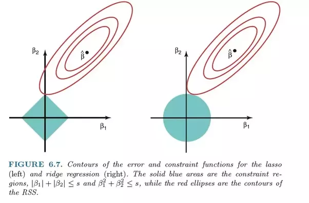
Comparison of errors in lasso regression (left) and ridge regression (right). Since Ridge Regression uses L2 regularization, its area resembles a circle, while L1 lasso regularization draws straight lines. Free image. Source
In the lasso, improvement from error 5 to error 4 is weighted in the same way as improvement from 4 to 3, and also from 3 to 2, from 2 to 1, and from 1 to 0. Therefore, more coefficients reach zero and more features are eliminated.
However, in ridge regression, the improvement from error 5 to error 4 is calculated as 5² - 4² = 9, while improvement from 4 to 3 is weighted only as 7. Gradually, the reward for improvement decreases; therefore, fewer features are eliminated.
Ridge regression is best suited for situations where we want to prioritize a large number of variables, each of which has a small effect. If your model needs to account for multiple variables, each of which has a medium to large effect, the lasso is the best choice.
Implementation
Ridge regression
sklearncan be implemented as follows (see below). As with lasso regression, sklearnthere is an implementation to cross-validate the selection of the best of many trained models.
from sklearn.linear_model import RidgeCV
model = Ridge()
model.fit(X_train, y_train)
5. ElasticNet regression
Theory
ElasticNet aims to combine the best of Ridge Regression and Lasso Regression by combining L1 and L2 regularization.
Lasso and Ridge Regression are two different regularization methods. In both cases, λ is the key factor that controls the size of the fine:
- λ = 0, , .
- λ = ∞, - . , , .
- 0 < λ < ∞, λ , .
To the λ parameter, ElasticNet regression adds an additional parameter α , which measures how "mixed" the regularizations L1 and L2 should be. When α is 0, the model is pure ridge regression, and when α is 1, it is pure lasso regression.
The “mixing factor” α simply defines how much L1 and L2 regularization should be considered in the loss function. All three popular regression models - Ridge, Lasso, and ElasticNet - aim to reduce the size of their coefficients, but each acts differently.
Implementation
ElasticNet can be implemented using sklearn's cross-validation model:
from sklearn.linear_model import ElasticNetCV
model = ElasticNetCV()
model.fit(X_train, y_train)
What else to read on the topic: