✍️ 🕗 👩‍🎨 Quantum computing in bioinformatics 🌨️ 🚚 👩🏽‍🎓

Quantum computers, by definition, can solve many problems exponentially faster than classical computers. It must be admitted that we have not yet reached the emergence of useful quantum computing, but when we can solve this problem, then the benefits recovered will affect almost all scientific disciplines. In this review, we look at how modern quantum algorithms can revolutionize computational biology and bioinformatics.

From the ability to process huge amounts of information and use machine learning algorithms much more efficiently, to quantum modeling algorithms that can improve computations (both qualitatively and quantitatively) for the design of new drugs, predicting protein structure, analyzing various processes in a biological organism, and etc. These mind-boggling perspectives are subject to overwhelming info hype today, which means it's important to highlight the caveats and challenges in this new technology.

Warning: The review is based on an article by a group of European researchers from the UK and Switzerland (Carlos Outeiral, Martin Strahm, Jiye Shi, Garrett M. Morris, Simon C. Benjamin, Charlotte M. Deane. "The prospects of quantum computing in computational molecular biology", WIREs Computational Molecular Science published by Wiley Periodicals LLC, 2020). The most difficult parts of the article related to sophisticated mathematical models will not be included in the review. But the material is initially complex, and the reader is required to have knowledge of mathematics and quantum physics.

But if you intend to start studying the application of quantum technologies in bioinformatics, then in order to first get into the topic, it is suggested to listen to a short talk by Viktor Sokolov, Senior Researcher at M&S Decisions, which outlines some modern problems of drug modeling:

Introduction

Since the advent of high performance computing, algorithms and mathematical models have been used to solve problems in the biological sciences - from studying the complexity of the human genome to modeling the behavior of biomolecules. Computational methods are regularly used today to analyze and extract important information from biological experiments, as well as to predict the behavior of biological objects and systems. In fact, 10 of the 25 most cited scientific papers deal with computational algorithms used in biology [see p. here ], including quantum modeling [ here , here , here and here ], sequence alignment [ here , here andhere ], computational genetics [see. here ] and X-ray diffraction in data processing [cf. here and here ].

Despite this progress, many problems in biology remain insoluble from the point of view of their solution using existing computational technologies. The best algorithms for tasks such as predicting protein folding, calculating the binding affinity of a ligand to a macromolecule, or finding the optimal large-scale genomic alignment requires computational resources that go beyond even the most powerful supercomputers available today.

The solution to these problems may lie in a paradigm shift in computing technology. In the 1980s independently, Richard Feynman [see here ] and Yuri Manin [see. here ] proposed to use quantum mechanical effects to create a new, more powerful generation of computers.

Quantum theory has proven to be a highly successful description of physical reality and has led, since its inception in the early 20th century, to advances such as lasers, transistors, and semiconductor microprocessors. The quantum computer uses the most efficient algorithms, using operations that are not possible in classical machines. Quantum processors do not run faster than classical computers, but they work in a completely different way, achieving unprecedented speedups, avoiding unnecessary computation. For example, calculating the total electron wave function of the average drug molecule on any modern supercomputer using conventional algorithms is expected to take longer than the full age of our universe [see Ref. here], while even a small quantum computer can solve this problem within a few days. Encouraged by such a promise of quantum advantage, engineers and scientists are continuing their quest for a quantum processor. However, the technical difficulties in manufacturing, managing and protecting quantum systems are incredibly complex, and the first prototypes have only appeared in the last decade.

It is important to note that the technical problems of building quantum computers have not stopped the development of quantum computing algorithms. Even in the absence of hardware, algorithms can be analyzed mathematically, and the advent of high-performance quantum computer simulators, as well as early prototypes in the past few years, has allowed further research to advance.

Several of these algorithms have already shown promising potential applications in biology. For example, the quantum phase estimation algorithm allows for exponentially faster eigenvalue calculations [see. here ], which can be used to understand large-scale correlation between parts of a protein or to determine the centrality of a graph in a biological network. The quantum Harrow-Hasidim-Lloyd (HHL) algorithm [cf. here ] can solve some linear systems exponentially faster than any known classical algorithm, and can also apply statistical learning methods with a much faster adaptation process and the ability to manage large amounts of data.

Quantum optimization algorithms have a wide field of application in the field of protein folding and selection of conformers, as well as in problems associated with finding minima or maxima [see. here ]. Finally, technology has recently been developed to simulate quantum systems that promise, for example, to produce accurate predictions of drug-receptor interactions [see Ref. here ] or to participate in the study and understanding of complex processes and chemical mechanisms such as photosynthesis [see. here ]. Quantum computing can significantly change the methods of biology itself, as classical computing did in its time.

Recent claims of quantum supremacy from Google [cf. here], although disputed by IBM [cf. here ], indicate that the era of quantum computing is not far off. The first processors using quantum effects to perform computations impossible for classical computer technology are expected within the next decade [see Ref. here ].

In this review, we'll break down the key points where quantum computing holds promise for computational biology. These reviews analyze the potential impact of quantum computing in a variety of areas, including machine learning [cf. here , here and here ], quantum chemistry [cf. here , here and here ] and drug synthesis [see.here ]. Also recently published was a report from the NIMH Workshop on Quantum Computing in Life Sciences [see here ].

In this review, we first give a brief description of what is meant by quantum computing and a short introduction to the principles of quantum information processing. We then discuss three main areas of computational biology, where quantum computing has already shown promising algorithmic developments: statistical methods, electronic structure calculations, and optimization. Some important topics will be left aside, for example, string algorithms that can affect sequence analysis [see. here ], medical imaging algorithms [see. here ], numerical algorithms for differential equations [here ] and other mathematical problems or methods for analyzing biological networks [ here ]. Finally, we discuss the potential impact of quantum computing on computational biology in the medium to long term.

1. Quantum information processing

Quantum computers promise to solve problems in the biological sciences, such as predicting protein-ligand interactions or understanding the co-evolution of amino acids in proteins. And it's not easy to solve, but to do it exponentially faster than you can imagine with any modern computer. However, this paradigm shift requires a fundamental change in our thinking: quantum computers are very different from their classical predecessors. The physical phenomena that underlie quantum advantage are often illogical and counterintuitive, and using a quantum processor requires a fundamental change in our understanding of programming. In this section, we present the principles of quantum information and how it is processed to perform computations.

We explain how information works differently in a quantum system, where it is stored in qubits, and how that information can be manipulated using quantum gates. Like variables and functions in a programming language, qubits and quantum gates define the basic elements of any algorithm. We will also examine why the creation of a quantum computer is technically extremely difficult and what can be achieved with the help of early prototypes that are expected in the coming years. This introduction will only cover the main points; for a comprehensive study read the book by Nielsen and Chuang [ here ].

1.1. Elements of quantum algorithms

1.1.1. Quantum information: an introduction to the qubit

The first problem in representing quantum computing is understanding how it processes information. In a quantum processor, information is usually stored in qubits, which are the quantum analog of classical bits. A qubit is a physical system, like an ion, limited by a magnetic field [see. here ] or a polarized photon [see. here ], but it is often spoken of in the abstract. Like Schrödinger's cat, a qubit can take not only states 0 or 1, but also any possible combination of both states. When a qubit is observed directly, it will no longer be in a superposition that collapses to one of the possible states, just as Schrödinger's cat is dead or alive after opening the box [see. here]. More importantly, when multiple qubits are combined, they can become correlated, and interactions with any of them have consequences for the entire collective state. The phenomenon of correlation between multiple qubits, known as quantum entanglement, is a fundamental resource for quantum computing.

In classical information, the fundamental unit of information is a bit, a system with two identifiable states, often denoted 0 and 1. A quantum analog, a qubit, is a two-state system, the states of which are labeled | 0⟩ and | 1⟩. We use Dirac's notation, where | *⟩ identifies a quantum state. The main difference between classical and quantum information is that a qubit can be in any superposition of states | 0⟩ and | 1⟩:

The complex coefficients α and β are known as amplitudes of states, and they are related to another key concept in quantum mechanics: the effect of physical measurement. Since qubits are physical systems, you can always come up with a protocol to measure their state. If, for example, the states | 0⟩ and | 1⟩ correspond to the states of the spin of an electron in a magnetic field, then measuring the state of a qubit is simply measuring the energy of the system. The postulates of quantum mechanics dictate that if the system is in a superposition of possible measurement results, then the act of measurement must change the state itself. The superposition system will fall apart at the measurement stage; the measurement thus destroys the information carried by the amplitudes in the qubit.

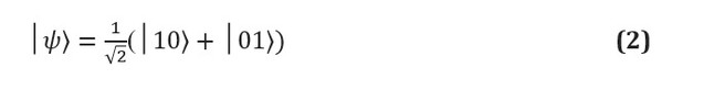
Important computational implications arise when we consider systems of multiple qubits that can experience quantum entanglement. Entanglement is a phenomenon in which a group of qubits are correlated, and any operation on one of these qubits will affect the overall state of all of them. A canonical example of quantum entanglement is the Einstein-Podolsky-Rosen paradox, presented in 1935 [cf. here ]. Consider a system of two qubits, where, since each of the individual qubits can take any superposition of states {| 0⟩ and | 1⟩}, the composite system can take any superposition of states {| 00⟩, | 01⟩, | 10⟩, | 11 ⟩} (And, accordingly, the system of N-qubits can take any of

2^{N}

$2^N$ binary strings, from {| 0 ... 0⟩ to | 1 ... 1⟩}. One of the possible superpositions of the system are the so-called Bell states, one of which has the following form: If we take a measurement on the first qubit, we can only observe | 0⟩ or | 1⟩, each of which will have a probability of 1/2. This does not make any changes for the single qubit case. If the outcome for the first qubit was | 0⟩, the system will collapse to the system | 01⟩, and therefore any measurement on the second qubit will give | 1⟩ with probability 1; similarly, if the first measurement was | 1⟩, the measurement on the second qubit would give | 0⟩. An operation (in this case, a measurement with the result "0") applied to the first qubit affects the results that can be seen when the second qubit is subsequently measured.

The existence of entanglement is fundamental to useful quantum computing. It has been proven that any quantum algorithm that does not use entanglement can be applied to a classical computer without a significant difference in speed [cf. here and here ]. Intuitively, reason is the amount of information that a quantum computer can manipulate. If the N qubit system is not entangled, then

2^{N}

$2^N$ amplitudes of its state can be described by the amplitudes of each one-bit state, that is, 2N amplitudes. However, if the system is entangled, all amplitudes will be independent, and the qubit register will form

2^{N}

$2^N$ -dimensional vector. The ability of quantum computers to manipulate vast amounts of information with multiple operations is one of the main advantages of quantum algorithms and underpins their ability to solve problems exponentially faster than classical computer technology.

1.1.2. Quantum gates

The information stored in qubits is processed using special operations known as quantum gates. Quantum gates are physical operations, such as a laser pulse directed at an ion qubit, or a set of mirrors and beam splitters through which a photon qubit must travel. However, gates are often viewed as abstract operations. The postulates of quantum mechanics impose some stringent conditions on the nature of quantum gates in closed systems, which allows them to be represented in the form of unitary matrices, which are linear operations that preserve the normalization of the quantum system.

In particular, a quantum gate applied to an entangled register of N qubits is equivalent to multiplying the matrix

2^{N}

$2^N$ ×

2^{N}

$2^N$ per input vector

2^{N}

$2^N$ . The ability of a quantum computer to store and perform computations of vast amounts of information is of the order of

2^{N}

$2^N$ - by manipulating multiple elements - of order N - forms the basis of its ability to provide a potentially exponential advantage over classical computers.

Essentially, quantum gates are any permitted operation in a qubit system. The postulates of quantum mechanics impose two strict constraints on the shape of quantum gates. Quantum operators are linear. Linearity is a mathematical condition that nevertheless has profound implications for the physics of quantum systems and, therefore, how they can be used for computation. If the linear operator is applied to the superposition of states

\hat{O}

$\hat{O}$ , the result is a superposition of the individual states, which are affected by the operator. In a qubit, this means: Linear operators can be represented as matrices, which are simply tables indicating the effect of a linear operator on each basis state. Figure 1 (c, d) shows a matrix representation of one of two qubit and two one-bit gates. However, not every matrix represents real quantum gates. We expect that quantum gates applied to a set of qubits will give a different real set of qubits, in particular, a normalized one (for example, in equation (3) we expect that

{| \overset{´}{α} |}^{2} + {| \overset{´}{β} |}^{2} = 1

$\left|\acute{\alpha}\right|^2+\left|\acute{\beta}\right|^2=1$

2^{N}

$2^N$ ×

2^{N}

$2^N$ is a fully valid N-qubit quantum gate.

In classical computation, there is only one non-trivial gate for one bit: the NOT gate, which converts 0 to 1 and vice versa. In quantum computing, there are an infinite number of 2 × 2 unitary matrices, and any of them is a possible one-qubit quantum gate. One of the early successes of quantum computing was the discovery that this vast array of possibilities could be realized with a set of universal gates affecting one and two qubits [see Ref. here]. In other words, given arbitrary quantum gates, there is a one- and two-qubit gates circuit that can drive it with arbitrary precision. Unfortunately, this does not mean that the approximation is effective. Most quantum gates can only be approximated by an exponential number of gates from our universal set. Even if these gates can be used to solve useful problems, their implementation will take an exponentially large amount of time and can negate any quantum advantage. FIGURE 1 (a) Comparison of a classical bit with a quantum bit or "qubit". While a classical bit can only take one of two states, 0 or 1, a quantum bit can take any state of the form

| ψ ⟩ = \cos \frac{Θ}{2} | 0 ⟩ + e^{i φ} \sin \frac{Θ}{2} | 1 ⟩

$|\psi⟩=\cos{\frac{\Theta}{2}}|0⟩+e^{i\varphi}\sin{\frac{\Theta}{2}}|1⟩$ ... Single qubits are often depicted using the Bloch sphere representation, where θ and ϕ are understood as azimuthal and polar angles in a sphere of unit radius. (b) A schematic of an ion trap qubit, one of the most common approaches to experimental quantum computing. Ion (often

^{43} C a^{+}

$^{43}Ca^+$ ) is held in a high vacuum by electromagnetic fields and exposed to a strong magnetic field. The hyperfine levels are separated according to the Zeeman effect, and the two selected levels are selected as states | 0⟩ and | 1⟩. Quantum gates are produced by appropriate laser pulses, often involving other electronic levels. This diagram was adapted from [see. here ]. (c) Diagram of a quantum circuit that implements X or the quantum of controlled negation (CNOT).

The representation and change in the Bloch sphere is shown. (d) Quantum circuit for generating the Bell state

\frac{1}{\sqrt{2}} (| 00 ⟩ + | 11 ⟩)

$\frac{1}{\sqrt2}(|00⟩+|11⟩)$ using a Hadamard gate and a CNOT (controlled negation) gate. The dotted line in the middle of the outline indicates the state after the Hadamard valve is applied.

1.2. Quantum hardware

Quantum algorithms can only solve interesting problems if they run on the right quantum hardware. There are many competing proposals for the creation of a quantum processor based on trapped ions [see. here ], superconducting circuits [see. here ] and photonic devices [see. here]. However, they all face a common problem: computational errors that can literally ruin the computational process. One of the cornerstones of quantum computing is the discovery that these errors can be eliminated with quantum error-correcting codes. Unfortunately, these codes also require a very large increase in the number of qubits, so significant technical improvements are needed to achieve fault tolerance.

There are many sources of error that can affect a quantum processor. For example, the connection of a qubit with its environment can lead to the collapse of the system into one of its classical states - a process known as decoherence.... Small fluctuations can transform quantum gates, which eventually lead to different results than expected. The least error-prone gates to date have been recorded in a trapped ion processor, with a frequency of one error per

10^{6}

$10^6$ one-qubit gates and with 0.1% error rate for two-qubit gates [ here and here ]. By comparison, a recent work by Google reported fidelity of 0.1% for single-qubit gates and 0.3% for two-qubit gates in a superconducting processor [see Ref. here ]. Given that the failure of one gateway can ruin the calculation, it is easy to see that propagation of error can make the calculation meaningless after a small sequence of elements.

One of the main directions of quantum computing is the development of quantum error-correcting codes. In the 1990s, several research groups proved that these codes can achieve fault-tolerant computations, provided the gate error rates are below a certain threshold, which depends on the code [see. here , here , here and here ]. One of the most popular approaches, surface code, can operate with error rates approaching 1% [see Ref. here ].

Unfortunately, quantum error correction codes require a large number of real physical qubits to encode the abstract logical qubit that is used for computation, and this overhead increases with the error rate. For example, a quantum algorithm for factorizing prime numbers [see. here ] could quietly decompose a 2000-bit number using about 4000 qubits and, at 16 GHz, this process would take about one day of work. Assuming an error rate of 0.1%, the same algorithm, using the surface code to correct environmental errors, would require several million qubits and the same amount of time [see Ref. here]. Considering that the current record for a controlled, programmable quantum processor is 53 qubits [see. here ], there is still a long way to go in this research direction.

Many groups have made efforts to develop algorithms that can be run on so-called medium-scale noise quantum processors [cf. here ]. For example, variational algorithms combine a classical computer with a small quantum processor, performing a large amount of short quantum computations that can be accomplished before the noise becomes significant.

These algorithms often use a parameterized quantum circuit, which performs a particularly difficult task, and use a classical computer to optimize the parameters. The resolution method is an error reduction region in which, instead of achieving fault tolerance, an attempt was made to minimize errors with minimal effort to drive larger gate circuits. There are a number of approaches that include the use of additional operations to discard runs with errors [see. here ] or manipulation of the error rate to extrapolate to the correct result [cf. here and here]. Although the main applications will require very large fault-tolerant quantum computers; devices available over the next decade are expected to solve these problems [see here ].

2. Statistical methods and machine learning

In computational biology, where the goal is often to collect massive amounts of data, statistical methods and machine learning are key techniques. For example, in genomics, hidden Markov models (HMM) are widely used to annotate information about genes [see. here ]; in drug discovery, a wide range of statistical models have been developed to evaluate molecular properties or to predict ligand-protein binding [see. here ]; and in structural biology, deep neural networks have been used both to predict protein connections [see. here ] and secondary structure [see. here ], and more recently also three-dimensional protein structures [see. here ].

Training and developing such models is often computationally intensive. A major catalyst for recent advances in machine learning has been the realization that general-purpose graphics processing units (GPUs) can dramatically speed up learning. By providing exponentially faster algorithms for machine learning, quantum computing models can provide similar interest in application focus to scientific problems.

In this section, we will explain how quantum computing can speed up numerous statistical learning methods.

2.1. Advantages and Disadvantages of Quantum Machine Learning

We first look at the benefits that a quantum computer provides for machine learning. Except for idealized examples, quantum computers can learn no more information than a classical computer [cf. here ]. However, in principle they can be much faster and capable of processing much more data than their classical counterparts. For example, the human genome contains 3 billion base pairs, which can be stored in 1.2 ×

10^{10}

$10^{10}$ classical bits - approximately 1.5 gigabytes. A register of N qubits includes

2^{N}

$2^N$ amplitudes, each of which can represent a classic bit by setting the k-th amplitude to 0 or 1 with an appropriate normalization factor. Hence, the human genome can be stored in ~ 34 qubits. While this information cannot be extracted from a quantum computer, until a certain state is prepared, certain machine learning algorithms can be executed on it. More importantly, doubling the register size to 68 qubits leaves enough room to store the complete genome of every living person in the world. The presentation and analysis of such huge amounts of data would be quite consistent with the capabilities of even a small fault-tolerant quantum computer.

Operations to process this information can also be exponentially faster. For example, multiple machine learning algorithms are limited to long-term inversion of the covariance matrix with a penalty

O {(N}^{3})

$\mathcal{O}{(N}^3)$ on the dimensions of the matrix. However, the algorithm proposed by Harrow, Hassidim, and Lloyd [cf. here ], allows you to invert the matrix into

O (\log N)

$\mathcal{O}(\log{N})$ under some conditions. The key insight is that, unlike graphics accelerators, which accelerate computations through massive parallelism, quantum algorithms have the advantage of the complexity of the computational algorithms directly used. In some cases, especially with the current exponential acceleration, midsize quantum computers can solve learning problems available only to the largest classical supercomputers available today.

Improved storage and processing of data has secondary benefits. One of the strengths of neural networks is their ability to find concise representations of data [see. here]. Since quantum information is more general than classical information (after all, the states of a classical bit are subdivided into eigenstates | 0⟩ and | 1⟩, or a qubit), it is entirely possible that quantum machine learning models can better assimilate information than classical models ... On the other hand, quantum algorithms with logarithmic time complexity also improve data confidentiality [see. here ]. Since training the model requires

O (\log N)

$\mathcal{O}(\log{N)}$ , and

O (N)

$\mathcal{O}\ (N)$ requires matrix reconstruction, for a large enough dataset it is impossible to recover a significant part of the information, although effective training of the model is still possible. In the context of biomedical research, this can facilitate data exchange while ensuring confidentiality.

Unfortunately, although quantum machine learning algorithms on paper can vastly outperform classical counterparts, practical difficulties still remain. Quantum algorithms are often subroutines that transform input into output. Problems arise precisely at these two stages: how to prepare adequate input and how to extract information from output [see. here ]. Suppose, for example, that we are using the HHL algorithm [see. here ] to solve a linear system of the form

A \vec{x} = \vec{b}

$A\vec{x}=\vec{b}$ ... At the end of the subroutine, the algorithm will output the qubit register in the following state: Here

u_{j}

$u_j$ and

μ_{j}

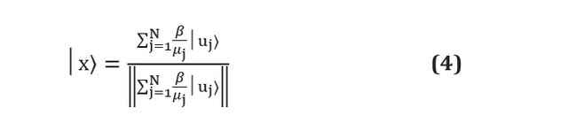
$\mu_j$ Are the eigenvectors and eigenvalues of A, and

β_{j}

$\beta_j$ - j-th coefficient

\vec{b}

$\vec{b}$ is expressed in terms of the eigenvectors of A, and the denominator is simply a normalization constant. It can be seen that this corresponds to the coefficients

\vec{x}

$\vec{x}$ , which are stored in the amplitudes of various states as

x_{j} = β_{j} λ_{j}^{- 1}

$x_j=\beta_j\lambda_j^{-1}$ and are not directly accessible. Measurement of the qubit register will lead to its collapse into one of the states of the eigenvector, and to re-estimate the amplitudes of each

x_{j}

$x_j$ measurements required

O (2^{N})

$\mathcal{O}\ (2^N)$ , which in the first place outweighs any advantage of the quantum algorithm.

HHL and many other algorithms are only useful for computing the global property of a solution, such as the expected value. In other words, HHL cannot provide a solution to a system of equations or invert a matrix in logarithmic time, if we are not interested only in the global properties of the solution, which can be obtained using several physically observable measurements. This limits the use of some routines, but there have been many suggestions to work around this problem.

Entering information into a quantum computer is a much bigger problem. Most quantum machine learning algorithms assume that the quantum computer has access to the dataset in the form of a superposition state; for example, there is a qubit register that is in a state of the form: Here - | bin (j) is a state that acts as an index, and

α_{j}

$\alpha_j$ Is the corresponding amplitude. This can be used, for example, to store the elements of a vector or matrix. In principle, there is a quantum circuit that can prepare this state by acting in, say, state | 0 ... 0⟩. However, its implementation can be very difficult, since we expect that the approximation of a random quantum state will be exponentially difficult and will destroy any possible quantum advantage.

Most quantum algorithms assume access to quantum random access memory (QRAM) [see. here ], which is a black box device capable of constructing this superposition. Although some drawings have been proposed [see. here and here], as far as we know, there is no working device yet. Moreover, even if such a device were available, there is no guarantee that it will not create bottlenecks that outweigh the benefits of the quantum algorithm. For example, a recent schema-based proposal for QRAM [cf. here ] shows the unavoidable linear cost of the number of states that outweighs any log-time algorithm. Finally, even if QRAM introduces no additional cost, classic preprocessing will still need to be done - for the genome example, access to 12 exabytes of classic storage would be required.

Finally, we must emphasize that quantum machine learning algorithms are not free from one of the most common problems in practical applications: lack of relevant data. The availability of large amounts of data is critical to the success of many practical applications of AI in molecular science, such as de novo molecular development [see Ref. here ]. However, the power of quantum algorithms can be useful as scientific and technological developments such as the emergence of self-managed laboratories [see Ref. here ] provide more and more data.

Quantum machine learning has the potential to transform the way we process and analyze biological data. However, the current practical challenges of implementing quantum technologies are still significant.

2.2. Quantum machine learning algorithms

2.2.1. Learning without a teacher

Unsupervised learning includes several techniques for extracting information from untagged datasets. In biology, where next-generation sequencing and great international collaboration have stimulated the collection of data, these methods have found widespread use, for example, to identify links between families of biomolecules [see. here ] or annotated genomes [see. here ].

One of the most popular unsupervised learning algorithms is principal component analysis (PCA), which attempts to reduce the dimensionality of data by finding linear combinations of features that maximize variance [cf. here]. This method is widely used in all kinds of high-dimensional datasets, including RNA microarray and mass spectrometry data [see. here ]. A quantum algorithm for PCA was proposed by a group of researchers [see. here ]. Essentially, this algorithm builds a data covariance matrix in a quantum computer and uses a subroutine known as quantum phase estimation to compute the eigenvectors in logarithmic time. The output of the algorithm is a superposition state of the form: Here

| η_{j} ⟩

$|\eta_j⟩$ Is the j-th main component, and

r_{j}

$r_j$ - the corresponding eigenvalue. Since the PCA is interested in large eigenvalues, which are the main components of variance, the final state measurement will give a suitable principal component with high probability. Repeating the algorithm several times will provide a set of core components. This procedure is capable of reducing the dimension of the vast amount of information that can be stored in a quantum computer.

A quantum algorithm has also been proposed for a particular method for analyzing topological data, namely for stable homology [see. here ]. Topological data analysis attempts to extract information using topological properties in the geometry of datasets; it was used, for example, in the study of data aggregation [see.here ] and network analysis [see. here ]. Unfortunately, the best classical algorithms have an exponential dependence in the dimension of the problem, which limits its application. Algorithm of Lloyd et al. also uses a quantum phase estimation routine to exponentially speed up matrix diagonalization, reaching complexity

O (N^{5})

$\mathcal{O}(N^5)$ ... The presence of an efficient algorithm for performing topological analysis can stimulate its application for the analysis of problems in biological sciences.

2.2.2. Supervised learning

Supervised learning refers to a set of methods that can be used to make predictions based on labeled data. The goal is to build a model that can classify or predict the properties of invisible examples. Supervised learning is widely used in biology to solve problems as diverse as predicting the binding affinity of a ligand for a protein [see. here ] and diagnosis of diseases using a computer [see. here ]. Let's look at three supervised learning approaches.

Support Vector Machine(English support vector machine - SVM) is a machine learning algorithm that finds the optimal hyperplane separating data classes. SVM has been widely used in the pharmaceutical industry to classify small molecule data [cf. here ]. Depending on the kernel, SVM training usually takes from

O (N^{2})

$\mathcal{O}(N^2)$ before

O (N^{3})

$\mathcal{O}(N^3)$ ... Rebentrost [see. here ] presented a quantum algorithm that can train an SVM with a polynomial kernel in

O (l o g N)

$\mathcal{O}(logN)$ , and later it was extended to the core of the radial basis function (RBF) [see. here ]. Unfortunately, it is not clear how to implement the non-linear operations that are widely used in SVM, given that quantum operations are limited to be linear. On the other hand, a quantum computer allows other kinds of nuclei that cannot be realized in a classical computer [see. here ].

Gaussian Process Regression (GP) is a technique commonly used to build surrogate models, such as in Bayesian optimization [see p. here ]. GPs are also widely used to create quantitative structure-activity relationship (QSAR) models of drug properties.here ], and recently also for modeling molecular dynamics [see. here ]. One of the disadvantages of GP regression is the high value

O (N^{3})

$\mathcal{O}(N^3)$ inversion of the covariance matrix. Zhao and colleagues [see. here ] suggested using the HHL algorithm for linear systems to invert this matrix, achieving exponential acceleration (as long as the matrix is sparse and well conditioned) - a property that is often achieved by covariance matrices. More importantly, this algorithm has been extended to compute the logarithm of the limiting likelihood [cf. here ], which is an important step for hyperparameter optimization.

One of the most common methods in computational biology is the hidden Markov model (HMM), which is widely used in computational gene annotation and sequence alignment [cf. here]. This method contains a number of hidden states, each of which is associated with a Markov chain; transitions between hidden states lead to changes in the underlying distribution. Basically, HMM cannot be directly implemented in a quantum computer: sampling requires some kind of measurement that will disrupt the system. However, there is a formulation in terms of open quantum systems, that is, a quantum system that is in contact with the environment, which allows a Markov system [see. here ]. While no improvements have been proposed to the classical Baum-Welch algorithm for training HMMs, quantum HMMs have been found to be more expressive: they can reproduce a distribution with fewer hidden states [cf. here]. This could lead to wider application of the method in computational biology.

2.2.3. Neural networks and deep learning

Recent developments in machine learning have been stimulated by the discovery that multiple layers of artificial neural networks can detect complex structures in raw data [see p. here ]. Deep learning has begun to permeate every scientific discipline, and in computational biology, its advances include the accurate prediction of protein bonds. here ], improved diagnosis of some diseases [see. here ], molecular design [cf. here ] and modeling [see. here and here ].

Given the significant advances in the study of neural networks, significant work has been done to develop quantum analogs that can drive further advances in technology.

The name artificial neural network often refers to a multilayer perceptron of a neural network, where each neuron takes a weighted linear combination of its inputs and returns the result through a non-linear activation function. The main challenge in developing a quantum analog is how to implement a nonlinear activation function using linear quantum gates. There have been a lot of suggestions lately, and some ideas include measurements [cf. here , here and here ], dissipative quantum gates [ here], quantum computing with a continuous variable [ here ] and the introduction of additional qubits for constructing linear gates that simulate nonlinearity [see. here ]. These approaches aim to implement a quantum neural network that is expected to be more expressive than a classical neural network due to the greater power of quantum information. The advantages or disadvantages of scaling the training of a multilayer perceptron in a quantum computer are unclear, although the focus is on the possible enhanced expressiveness of these models.

A huge amount of recent effort has focused on Boltzmann machines, recurrent neural networks capable of acting as generative models. Once trained, they can generate new patterns similar to the training set.

Generative models have important applications, for example, in molecular design de novo [cf. here and here ]. Although Boltzmann machines are very powerful, it is necessary to solve the complex problem of sampling from the Boltzmann distribution in order to compute gradients and conduct training, which limits their practical application. Quantum algorithms have been proposed using the D-Wave machine [see. here , here and here ] or a circuit algorithm [see.here ]; this sample from the Boltzmann distribution is quadratically faster than is possible in the classical version [see. here ].

Recently, a heuristic for efficient training of quantum Boltzmann machines was proposed, based on the thermalization of the system [see. here ]. Moreover, in some works, quantum implementations of generative adversarial networks (GANs) have been proposed [see. here , here and here ]. These developments involve improving generative models as quantum computing hardware develops.

3. Effective simulation of quantum systems

According to the models, chemistry is regulated by electron transfer. Chemical reactions, as well as interactions between chemical entities, are also controlled by the distribution of electrons and the free energy landscape they form. Problems such as predicting ligand binding to a protein or understanding the catalytic pathway of an enzyme boil down to understanding the electronic environment. Unfortunately, modeling these processes is extremely difficult. The most efficient algorithm for calculating the energy of a system of electrons, full configuration interaction (FCI), which scales exponentially as the number of electrons grows, and even molecules with several carbon atoms are barely available for computational research [see. here]. Although there are many approximate methods, deeply and extensively described in publications on density functional theory [see. here and here ], they can be imprecise and even abruptly fail in many situations of interest, such as the simulation of the transient response state [cf. here ]. An accurate and efficient algorithm for studying electronic structure would provide a better understanding of biological processes and also open up opportunities for the development of next generation biological interactions.

Quantum computers were originally proposed as a method for more efficient modeling of quantum systems. In 1996, Seth Lloyd demonstrated that this is possible for certain kinds of quantum systems [ here], and a decade later, Alan Aspuru-Guzik and colleagues showed that chemical systems are one such case [ here ]. Over the past two decades, there has been significant research into fine-tuning modeling methods for chemical systems that can calculate properties of research interest.

3.1. Advantages and Disadvantages of Quantum Simulation

In principle, a quantum computer is able to efficiently solve a fully correlated electronic structure problem (FCI equations), which will be the first step to accurately estimate binding energies, as well as to simulate the dynamics of chemical systems. Classical computational chemistry has focused almost exclusively on approximate methods, which have been useful, for example, to estimate the thermochemical quantities of small molecules [ here], but this may not be enough for processes associated with breaking or forming bonds. In contrast, quantum processors can potentially solve an electronic problem by directly diagonalizing the FCI matrix, giving an accurate result within a certain basis set and thus solving many of the problems arising from incorrect descriptions of the physics of molecular processes (for example, polarization of ligands) ... Moreover, unlike classical approaches, they do not necessarily require an iterative process, although the initial assumption is still important.

Although quantum computers are not as deeply studied, they also overcome the limiting approximations that were needed in classical computing. For example, the formulation of quantum simulation in real space automatically takes into account the nuclear wave function in the absence of the Born-Oppenheimer approximation [ here ]. This makes it possible to study the non-adiabatic effects of some systems that are known to be important for DNA mutation [see. here ] and the mechanism of action of many enzymes [ here ]. Applications of quantum computing for relativistic system modeling have also been proposed [see. here ], which are useful for studying transition metals that appear in the active centers of many enzymes.

In an article by Reicher and colleagues [see here ] the concept of the time scale for calculating electronic structures in a quantum computer is revealed. The authors considered the cofactor FeMo of the nitrogenase enzyme, the mechanism of nitrogen fixation of which has not yet been studied and is too complex to be studied using modern computational approaches. The minimum baseline FCI calculation for FeMoCo will take several months and about 200 million qubits of the highest class available today. However, these estimates must change with the rapid development of technology. Over the 3 years since publication, algorithmic advances have already reduced the time requirements by several orders of magnitude [see. here]. In addition to the more powerful methods of electronic structure, fast versions of modern approximate methods that have been investigated recently [cf. here and here ] can significantly speed up prototyping, which could be useful, for example, when studying the coordinates of reactions of enzymatic reactions, the area of which is a problem for computational enzymology [ here ]. Moreover, with a better understanding of intermolecular interactions catalyzed by access to fully correlated computation or access to faster bandwidth that improves parameterization, quantum modeling can significantly improve non-quantum modeling techniques such as force fields.

One final point to watch out for is that unlike other areas of algorithm research, such as learning with quantum machines, there are a number of short-term quantum simulation algorithms that can be run on undemanding, pre-existing hardware. Numerous experimental groups around the world have reported successful demonstrations of these algorithms [ here , here , here and here ].

Unfortunately, there are also some drawbacks to quantum systems modeling. As discussed above, it is very difficult to extract information from a quantum computer. Reconstructing the entire wave function is more difficult than calculating it in the classical way. This is an important disadvantage for chemical problems, where arguments based on electronic structure are the main source of understanding. However, compared to machine learning, the advantages far outweigh the disadvantages, and quantum simulation is expected to be one of the first useful applications of practical quantum computing [see Ref. here ].

3.2. Fault Tolerant Quantum Computing

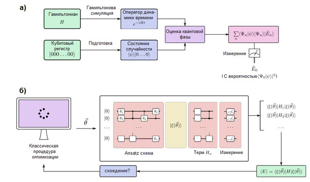
FIGURE 2. (a) A quantum simulation algorithm in a fault-tolerant quantum computer. The qubits are divided into two registers: one is prepared in the state

| ψ ⟩

$|\psi⟩$ , which resembles the target wave function, while the other remains in the state

| 0...0 ⟩

$|0...0⟩$ ... The quantum phase estimation (QPE) algorithm is used to find the eigenvalues of the time evolution operator

e^{- i H t}

$e^{-iHt}$ , which is prepared using the methods of Hamiltonian modeling. After QPE, the measurement of a quantum computer gives the ground state energy with probability

{| ⟨ Ψ_{0} | ψ ⟩ |}^{2}

$\left|\left\langle\Psi_0\middle|\psi\right\rangle\right|^2$ so it is important to prepare the state of the guess

| ψ ⟩

$|\psi⟩$ with non-zero overlap with the true wave function. (b) A variational quantum simulation algorithm in a short-term quantum computer. This algorithm combines a quantum processor with classical optimization routines to perform several short runs that are fast enough to avoid errors. A quantum computer prepares a state of guesswork

| ξ (\vec{θ}) ⟩

$\left|\xi\left.(\vec{\theta})\right\rangle\right.$ with a quantum ansatz chain depending on several parameters

{θ_{k}}

$\left\{\theta_k\right\}$ ... The individual terms of the Hamiltonian are measured one by one (or in commuting groups using more advanced strategies), giving an estimate of the expected energy for a particular vector of parameters. Then the parameters are optimized by the classical optimization procedure until convergence. The variational approach has been extended to many algorithmic problems besides quantum simulation.

Quantum computers that can simulate large chemical systems must be fault-tolerant in order to execute arbitrarily deep algorithms without error. Such a quantum computer is capable of simulating a chemical system by mapping the behavior of its electrons to the behavior of its qubits and quantum gates. The quantum modeling process is conceptually very simple and is depicted in Figure 2 (a). We will prepare a register of qubits that can store the wave function and implement the unitary evolution of the Hamiltonian

e^{- i H t}

$e^{-iHt}$ using the methods of Hamiltonian modeling, which are discussed below. With these elements, a quantum subroutine known as quantum phase estimation is able to find the eigenvectors and eigenvalues of the system. Namely, if the qubit register is initially in state | 0⟩, the final state will be: In other words, the final state is a superposition of eigenvalues

| {\tilde{E}}_{j} ⟩

$\left|\left.{\widetilde{E}}_j\right\rangle\right.$ and eigenvectors

| n_{j} ⟩

$\left|\left.n_j\right\rangle\right.$ systems. The ground state is then measured with probability

{| ⟨ Ψ_{n} | 0 ⟩ |}^{2}

$\left|\left\langle\Psi_n\middle|0\right\rangle\right|^2$ ... To maximize this likelihood, a baseline is established as an easy to prepare but also physically motivated state that is expected to be similar to the exact ground state. A typical example is the Hartree-Fock state, although other ideas have been explored for strongly correlated systems [see Ref. here ].

There are two common ways of representing electrons in a molecule: grid-based and orbital or basic methods (see McArdle and colleagues for a full breakdown [ here ]). In basis set methods, the electron wave function is represented as a sum of Slater determinants of electron orbitals, which can be directly compared with the qubit register [ here andhere ]. This requires the choice of a basis and preliminary calculation of electronic integrals. On the other hand, in grid methods, the problem is formulated as a solution to an ordinary differential equation in a grid. The advantage of grid-based modeling is that no Bourne-Oppenheimer approximation or base set is required. However, they are not naturally antisymmetric, which is required by the Pauli principle from quantum mechanics, so it is necessary to provide antisymmetry using the sorting procedure [ here ]. Grid-based methods have been discussed in the context of chemical dynamics simulations [cf. here ] and calculating the thermal rate constant [see. here]. Despite the differences, the quantum modeling workflow is identical, as shown in Figure 2.

There are also several ways to construct the operator

e^{- i H t}

$e^{-iHt}$ ... We will present the simplest technique, Trotterization, also known as product formulation [see p. here ]; for a complete overview see [ here and here ]. Trotterization is based on the premise that the molecular Hamiltonian can be split as the sum of terms describing one- and two-electron interactions. If so, then the operator

e^{- i H t}

$e^{-iHt}$ can be implemented in terms of the corresponding operators for each term in the Hamiltonian using the Trotter - Suzuki formula [ here ]: For example, in the second quantization, each term in this expression will have the form or , where are the annihilation and creation operators, respectively. Explicit, detailed schema constructions representing these terms have been given by Whitfield and colleagues [cf. here ]. After calculating the members

h_{i j}

$h_{ij}$ and

g_{i j k l}

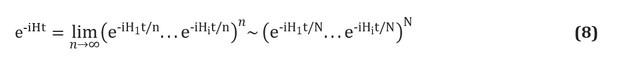
$g_{ijkl}$ known as electronic integrals, the quantity

e^{- i H t}

$e^{-iHt}$ completely determined. You can also use higher order Trotter – Suzuki formulas to reduce the error. There are many other Hamiltonian modeling techniques. Examples of powerful and sophisticated techniques are cubitization [ here ] and quantum signal processing [see Ref. here ], which have provably optimal asymptotic scaling, although it is unclear if this will lead to better practical applications.

4. Optimization problems

Many problems in computational biology and other disciplines can be formulated as finding the global minimum or maximum of a complex, multidimensional function. For example, it is believed that the native structure of a protein is the global minimum of its free energy hypersurface [see. here ]. In another area, identifying groups in a network of interacting proteins or biological objects is equivalent to finding an optimal subset of nodes [see. here]. Unfortunately, with the exception of a few simple systems, optimization problems are often very complex. Although there are heuristics for finding approximate solutions, they usually give only local minima, and in many cases even the heuristic is undecidable. The ability of quantum computers to speed up solutions to such optimization problems or to find better solutions has been investigated in detail.

The topic of optimization in a quantum computer is complex because it is often not obvious whether a quantum computer can provide any kind of acceleration. In this section, we will provide an overview of some of the ideas of quantum optimization. However, the guarantees of improvement are not so clear when compared to, for example, quantum simulation, which is expected to be beneficial in the long run.

4.1. Optimization in a quantum processor

Quantum adiabatic optimization is one of the most popular optimization approaches due to the presence of D-Wave machines [see. here ] that initially implement this approach. Adiabatic quantum computing [ here ] is based on the adiabatic theorem of quantum mechanics [cf. here]. According to this theorem, if a system is prepared in the ground state of the Hamiltonian, and this Hamiltonian changes rather slowly, the system will always remain in its instantaneous ground state. This can be used to perform computations by coding a problem (such as a scoring function that we hope to minimize) as a Hamiltonian, and gradually evolving towards this Hamiltonian from some original system that can be trivially prepared in its ground state. In general, adiabatic evolution is expressed as follows: Here

A (t)

$\mathcal{A}\left(t\right)$ and

B (t)

$\mathcal{B}\left(t\right)$ - functions such that

A (0) = B (T) = 1

$\mathcal{A}\left(0\right)=\mathcal{B}\left(T\right)=1$ and

A (T) = B (0) = 0

$\mathcal{A}\left(T\right)=\mathcal{B}\left(0\right)=0$ for a certain time T. For example, we could consider a linear annealing program with

A (t) = (1 - t / T)

$\mathcal{A}\left(t\right)=\left(1-t/T\right)$ and

B (t) = t / T

$\mathcal{B}\left(t\right)=t/T$ ... Many papers have been devoted to discussing the execution time of the adiabatic algorithm, but the general heuristic is that the execution time is maximally proportional to the inverse square of the minimum spectral gap (the smallest energy difference between the ground and first excited states) during adiabatic evolution

O (1 / Δ^{2})

$\mathcal{O}\left(1/\Delta^2\right)$ ... It is believed that adiabatic quantum computing (and quantum computing in general) is not able to effectively solve the class of NP-complete problems, or at least none of these methods has stood rigorous testing [see Ref. here ].

In principle, adiabatic quantum computing is equivalent to universal quantum computing [cf. here ]. This universality takes place only if evolution allows non-stochasticity, which means that the Hamiltonian has non-negative off-diagonal elements at some point in evolution. The most popular experimental implementation of adiabatic quantum computing, commercialized by D-Wave Systems Inc., uses stochastic Hamiltonians, and therefore it is not universal. There is some concern in the professional literature that this variety of quantum computing might be classically simulated [ here ], which means that exponential acceleration might not be possible. Despite these concerns, this technique has been widely used as a metaheuristic optimization technique and has recently been shown to outperform simulated annealing [see Ref. here ].

Quantum optimization has been studied outside of the adiabatic model. The e quantum approximate optimization algorithm (QAOA) [cf. here , here and here] Is a variational optimization algorithm in a quantum computer that has generated considerable interest in the literature. There have been several experimental implementations of QAOA in quantum processors, eg [see. here ] Figure 3. FIGURE 3. (a) Simulation of an adiabatic quantum computer implementing the simplified protein folding problem described [ here ]. The color encodes the decimal logarithmic probability of a particular binary string. At the end of the calculation, the two lowest energy solutions have a measurement probability close to 0.5. Evolution is never completely adiabatic in a finite time, and other binary strings have residual probabilities of measurement. (b)

Description of the adiabatic process of quantum computing. The potential driving the qubits changes slowly, causing them to rotate. Note that the Bloch sphere representation is incomplete as it does not display the correlations between different qubits that are required for quantum advantage. At the end of evolution, the qubit system is in a classical state (or a superposition of classical states), representing the solution with the lowest energy. (c) Energy levels during adiabatic quantum evolution. The amount of time required to ensure quasi-adiabatic evolution is determined by the minimum energy difference between the levels, which is indicated by the dashed line

4.2. Protein structure prediction

Prediction of protein structure without a matrix remains a major open unsolved problem in computational biology. The solution to this problem will find wide application in molecular engineering and drug design. According to the protein folding hypothesis, the native structure of a protein is considered a global minimum of its free energy [see. here ], although there are many counterexamples. Given the vast conformational space available even for small peptides, exhaustive classical simulations are unsolvable. However, many are wondering if quantum computing can help solve this problem.

The quantum computing literature focuses on the protein lattice model, where a peptide is modeled as a self-propelled lattice structure, although several other models have also recently begun to be applied in computational practice [cf. here ]. Each lattice site corresponds to a residue, and interactions between spatial neighboring sites contribute to the energy function. There are several schemes of energy contact, but only two have been used in quantum applications: the hydrophobic-polar model [see. here ], which considers only two classes of amino acids, and the Miyazawa-Jernigan model [cf. here], containing interactions for each pair of residues. While these models are a marked simplification, they have provided substantial insight into protein folding [see Ref. here ] and have been proposed as a crude tool for studying the conformational space before further detailed refinement [see. here and here ].

Almost all of the work has focused on adiabatic quantum computing, since even model peptides require a large number of qubits, and D-Wave quantum machines are the largest quantum devices available today.

However, in a recently published article by Fingerhat and colleagues [see here] an attempt was made to describe the use of the QAOA algorithm. Both methods have similar characteristics if the protein lattice problem is coded as the Hamilton operator. This method was first considered by Perdomo [see. here ], which suggested using a qubit register

D N l o g 2 N

$DNlog2N$ to encode the Cartesian coordinates of N amino acids on a D-dimensional cubic lattice with N sides. The energy function is expressed in a Hamiltonian containing terms to reward contacts with proteins: preserve the Primary structure and avoid amino acid matches. Shortly after this landmark article, another article appeared discussing the construction of more bit efficient models for a two-dimensional lattice [see. here ].

These encodings were tested on real hardware in 2012 when Perdomo and colleagues [see. here] calculated the lowest energy conformation of the PSVKMA peptide on a D-Wave quantum machine. Recently, Babay's research group extended the rotation and diamond encodings for 3D models and introduced algorithmic improvements that reduce the complexity and speed of movement of the Hamilton encoding [see Ref. here ]. They used a D-Wave 2000Q processor to determine the ground state of higolin (10 residues) on a square lattice and tryptophan (8 residues) on a cubic lattice, which are the largest peptides studied to date. These experimental implementations use a method in which a portion of the peptide is fixed. This allows large problems to be introduced into a quantum computer due to the possibility of research

2^{N}

$2^N$ the number of problem parameters studied.

Finding the lowest energy conformation in the lattice model is a difficult NP problem [see. here and here ], which means that under standard hypotheses there is no classical algorithm for solving. In addition, it is currently believed that quantum computers cannot offer exponential acceleration for NP-complete and more complex problems [cf. here ], although they may offer upscaling benefits that are known in the literature as "constrained quantum acceleration" [cf. here]. Recently, Outerel's research group applied numerical simulations to investigate this fact, concluding that there is evidence of limited quantum acceleration, although this result may require adiabatic machines using error correction or quantum simulations in fault-tolerant general-purpose machines [cf. here ].

Although most of the literature has focused on the protein lattice model, a recent article [ here ] attempted to use quantum annealing to sample rotamers in the Rosetta energy function [see Ref. here ]. Authors used D-Wave 2000Q processorto find a scaling that seemed nearly constant compared to classic simulated annealing. A very similar approach was presented by the Marchand group [see. here ] for a selection of conformers.

conclusions

A quantum computer can store and manipulate vast amounts of information, and execute algorithms at an exponentially faster rate than any classical computing technology. The potential of even small quantum computers can easily surpass the best supercomputers in existence today, which in the end, within the framework of certain tasks, can have a transformative effect for computational biology, promising to transfer problems from the category of unsolvable to difficult and complex to routine. The first quantum processors that can solve useful problems are expected to appear within the next decade. Therefore, understanding what quantum computers can and cannot do is a priority for every computational scientist.

Although we are just entering the era of practical quantum computing, we can already see the contours of a new quantum computational biology for the coming decades. We hope this review will generate interest among computational biologists for technologies that may soon change their field of experimentation and research. And specialists in quantum computing, in turn, will be able to help biologists significantly develop the level of computational biology and bioinformatics, from which many significant results are expected for all of humanity.

Quantum computing in bioinformatics