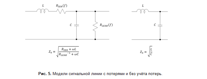
Characteristic impedance for a lossless line is expressed by the well-known formula:

where L L and C L are linear inductance and line capacitance (that is, per unit length). I think it will be useful to clarify where it comes from. Consider an extremely small section of a long two-wire transmission line through which an alternating current flows (Fig. 1). The current is alternating, so the instantaneous values of current, voltage between wires, linear electric charge density vary along the wires.
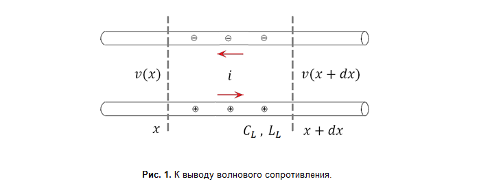
The charge conservation law for the wire section and the Faraday law for the circuit are as follows:

For a line without losses (R L = 0) and taking into account Φ L = L L ∙ i and q L = C L ∙ v we get:

These differential equations are reduced to waveform, for which we get:

where u is the speed of wave propagation, and the coefficient connecting the current in the wires and the voltage between the wires is the characteristic impedance. Here are some useful relationships (TD is the time delay of the line):

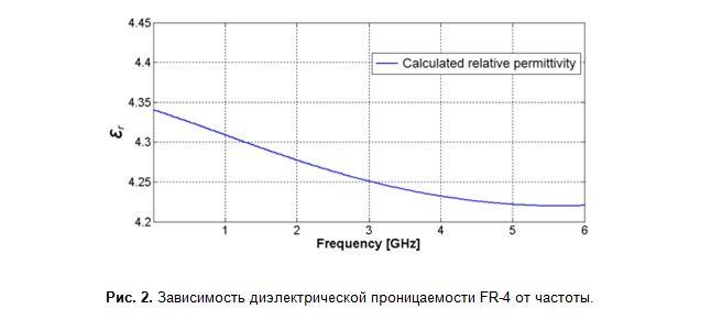
Capacitance and inductance depend on frequency, therefore the characteristic impedance changes with frequency. The influence of the skin effect on the inductance is limited to frequencies up to several tens of megahertz, in the upper frequency range it changes insignificantly. The value of the capacitance is affected by the dependence of the dielectric constant of the printed circuit board material on the frequency, and for microstrip lines, due to the asymmetry of the dielectric, also the effect of dispersion. The data for FR-4 fiberglass in different sources differ, however, as an estimate, it can be assumed that the dielectric constant decreases by 0.15-0.2 every decade (Fig. 2). The difference in data is due to the fact that FR-4 is a material class. It is composed of fiberglass and epoxy resin with significantly different dielectric constants (Figure 3).The more resin there is in the material, the less is the volume-averaged value of the dielectric constant of the glass fiber laminate. Hence, different values for different manufacturers. By the way, due to such anisotropy, the dielectric constant also depends on the direction - longitudinal or transverse, which affects the calculations for differential lines, since the field configuration will differ depending on the mode.

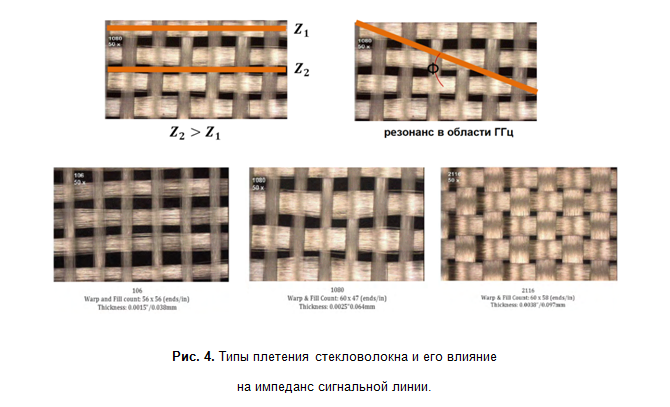
The mutual arrangement of fiberglass and conductor fibers also affects the characteristic impedance. If the conductor is located above the fiber, then its characteristic impedance will be slightly higher compared to the adjacent conductor, which fell into the gap between the fibers. If the conductor is directed at an angle to the fibers, then this leads to a periodic change in the characteristic impedance and resonance effects at frequencies in the region of tens of GHz. The degree of influence greatly depends on the type of fiberglass weaving (Fig. 4). This is why there are specialized materials for high frequency printed circuit boards, where the influence of these effects becomes significant. The parameters of such dielectrics have better stability over a wide frequency range and are much better documented.
With regard to losses (Fig. 5), for most practical cases the low-loss model is applicable, for which losses at high frequencies can be neglected R SER ≪ ωL, R LEAK ≫1⁄ωC. This simplification made it possible to develop efficient models that allow highly accurate calculation of signal line parameters using standard functions.
Planar signal lines were invented in the early 1950s, and accurate mathematical models were developed almost immediately for strip lines, and it took several decades to create an accurate microstrip analysis model. Harold Wheeler was one of the first (in 1965) to give exact solutions for special cases , which he generalized later (by 1977) . The reason is the asymmetry of the dielectric, which leads to a complex distribution of the electric field, which also depends on the frequency.
Naturally, this model was not the only one - and by 1988 there were enough of them to make it interesting to compare. This is donethe great and terrible Eric Bogatin. I came across this article when I was choosing a calculation model for a calculator. Then I got to Wheeler's publications, where there are many pages of cool mathematics with conformal transformations, and I realized that Bogatin had not read it carefully (or did not read it at all) and rude his model, which influenced the comparison results. Then this error migrated to the 2007th year. At the same time, Bogatin himself refers to the monograph "Microwave Transmission Line Impedance Data" by a certain M.A.R. Gunstan, but I no longer began to dig where the legs grow, recognizing Comrade Bogatin as the culprit (whom, by the way, I respect very much, Bogatin is strength).
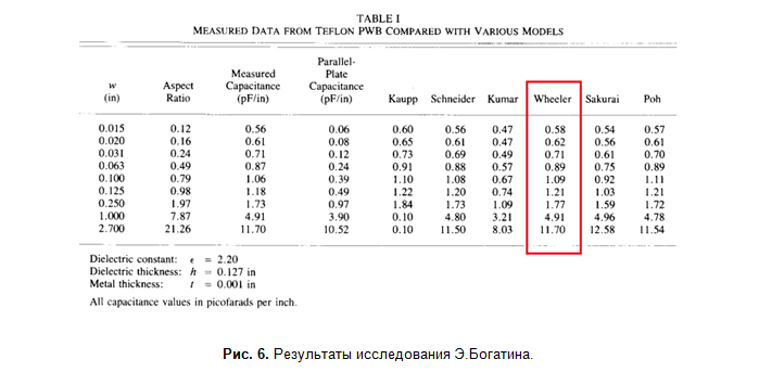
So what's the point. Bogatin experimentally measured the linear capacitance of microstrip lines of various widths (at a frequency of 1 kHz) and compared them with the calculated values (Fig. 6).
In all the models from which I studied the primary sources, analytical relations for the wave impedance are given. The capacity is calculated using the following ratio:

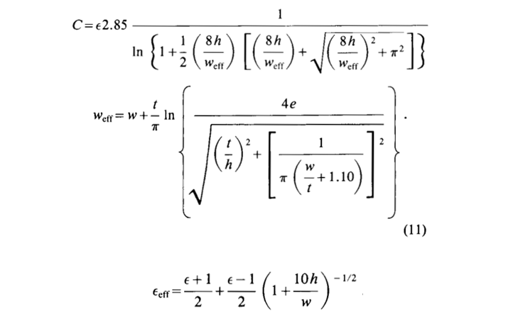
where ε r is the dielectric constant, c is the speed of light. The asymmetry of the dielectric leads to the fact that it is necessary to invent the effective value of the dielectric constant. Bogatin writes:
In the case of Wheeler [13], no model for the effective dielectric constant is offered. However, based on the suggestion by Gunsten [6], the plot for Wheeler's model uses the effective dielectric constant from Schneider's model.
and uses a hybrid Wheeler-Schneider model (result in pF / inch):
According to the results of the experiment, the model gives good accuracy and Bogatin praises his invented bicycle:
The combination of Wheeler's and Schneider's model is found to agree with previous published data and new data presented here to better than 3 percent, and is of a form suitable for use in a spread sheet. In addition to being useful for computer simulation of specific designs, this model can yield some useful insight to add to the intuition of fabrication and design engineers
Now let's turn to the original source. The formulas that Bogatin uses are simplified formulas for the case without a dielectric:
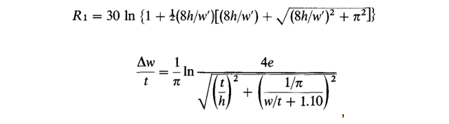
and the complete model looks like this:
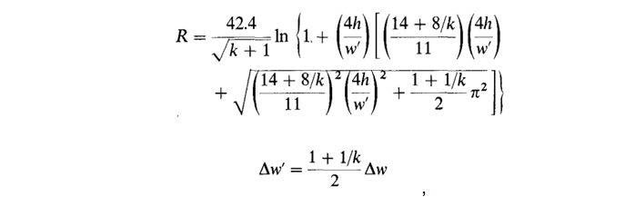
here, in Wheeler's notation, R is the wave resistance, k is the dielectric constant, R 1 = R (k = 1) is the resistance without a dielectric, ∆w is the width correction, taking into account the conductor thickness, ∆w 'is the correction taking into account the influence of the dielectric. Wheeler uses the notation k 'for the effective dielectric constant and gives it the following formula:

which is not as simple, of course, as that of Schneider, but nevertheless it is in the model. I repeated Bogatin's calculations, leaving the most accurate models: Schneider, Wheeler, their hybrid version - and added the results of the calculation using the Saturn PCB Toolkit calculator and the Hammerstead model . For clarity, I present both a graph and tabular data with an error relative to experimental data.
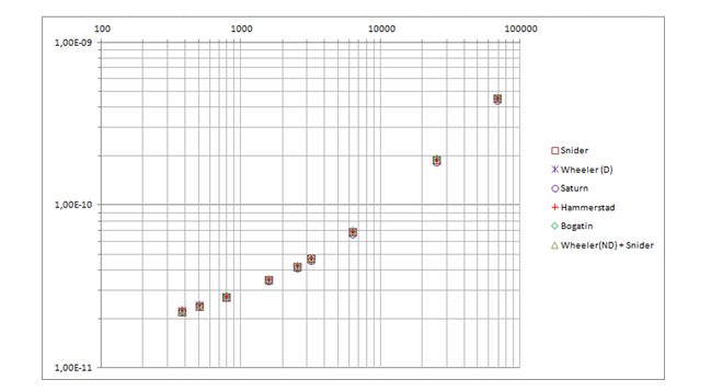
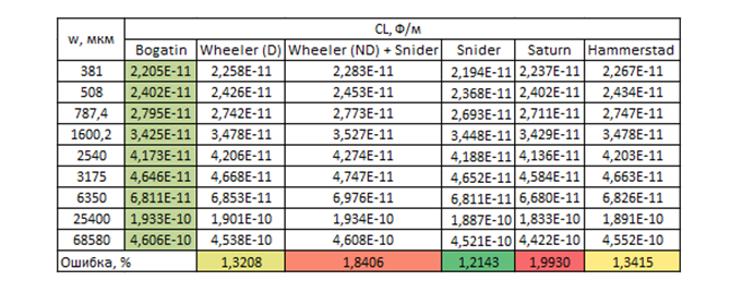
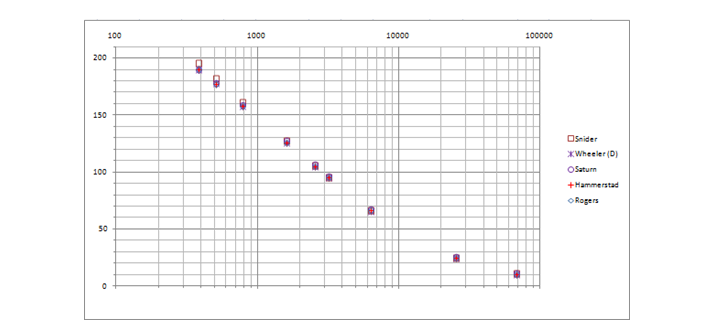
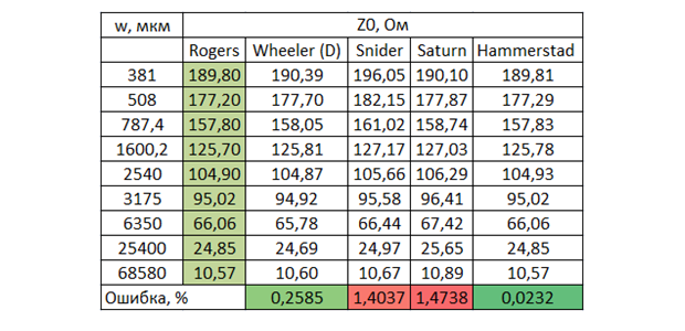
Taking into account the measurement errors and the dielectric constant of the base material (2.2 ± 1%), we can say that all models correlate well with the experimental data, it is not in vain that the researchers have adjusted the formulas for years. I expected more accuracy from Saturn, as it directly says that it uses a "not simple, but complex" formula and the accuracy is comparable to Sonnet 3D. In addition, there the thickness can only be selected in ounces, and this is either ½ oz. (18 microns), or 1 oz. (35 μm), and 1 mil (25.4 μm) is not specified. The values in the table are for ½ oz., Since they are closer to the experimental data obtained this way. It is also obvious that Wheeler's original model would have been more accurate on this sample of data, so I was annoyed with him. Especially considering thatthat just the same Schneider's model has a serious drawback - it does not take into account the effect of the conductor thickness, which has almost no effect on the capacitance, but is significant for the inductance and therefore the wave resistance itself. Unfortunately, Bogatin does not give the value of the wave impedance, so he usedcalculator from the reputable company Rogers. The Saturn this time is 1 oz. it gave a somewhat better accuracy, the logic of its work is not very clear to me yet. The graph shows that as the width decreases (where the effect of thickness increases), Schneider falls off. And Rogers, apparently, is based on the Hammerstead model. I originally made it on Wheeler , but since most of the advanced calculators are on Hammerstead, it will be possible to switch to this model in order to keep up with them (although the model does not have an explicit formula for synthesis, unlike Wheeler's).
Actually, on this I consider justice restored. Wheeler is power. Even Bogatin is sometimes wrong. So don't trust, check and double-check. Use the calculations for your signal lines. By the way. Please share in the comments if you use the calculation of the wave resistance and if so, with what help?
PS I am in the process of working on the calculator and am finalizing the book , now my hands have reached the free version - I have added all the improvements and fixes that were previously only made in full. Good luck to all!