👩🏻‍🤝‍👨🏽 💺 🤥 TensorFlow.js: Part 1: Using the Low-Level API to Approximate Linear Functions 🍱 🦋 😄

Python currently holds the dominant position for machine learning. However, if you are a JS developer and are interested in plunging into this world, then it is not necessary to include a new programming language in your arsenal, due to the advent of TensorFlow.js .

Benefits of using TensorFlow.js in a browser

interactivity - the browser has many tools for visualizing the ongoing processes (graphics, animation, etc.);
sensors - the browser has direct access to the device's sensors (camera, GPS, accelerometer, etc.);
security of user data - there is no need to send processed data to the server;
compatibility with models created in Python .

Performance

One of the main issues is performance.

Due to the fact that machine learning is, in fact, performing various kinds of mathematical operations with matrix-like data (tensors), the library for this kind of calculations in the browser uses WebGL. This significantly improves performance if the same operations were performed in pure JS. Naturally, the library has a fallback in case WebGL is not supported in the browser for some reason (at the time of this writing, caniuse shows that 97.94% of users have WebGL support).

To improve performance, Node.js uses native-binding with TensorFlow. Here, CPU, GPU and TPU ( Tensor Processing Unit ) can serve as accelerators

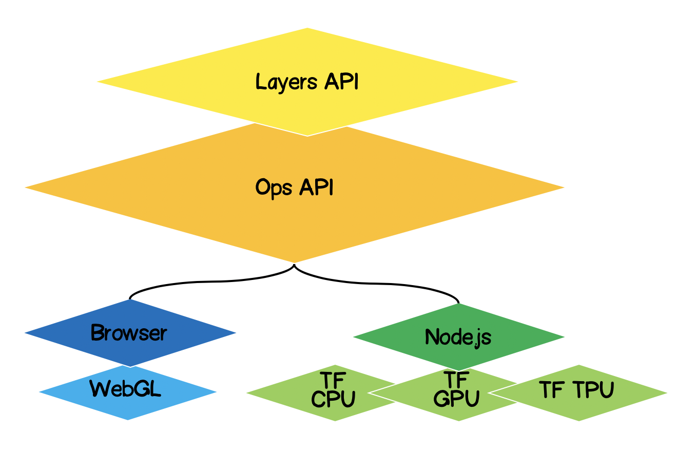
TensorFlow.js architecture

Lowest Layer - this layer is responsible for parallelizing computations when performing mathematical operations on tensors.
The Ops API - Provides API for performing mathematical operations on tensors.
Layers API - allows you to create complex models of neural networks using different types of layers (dense, convolutional). This layer is similar to the Keras Python API and has the ability to load pretrained Keras Python based networks.

Formulation of the problem

It is necessary to find the equation of the approximating linear function for a given set of experimental points. In other words, we need to find such a linear curve that would lie closest to the experimental points.

Solution formalization

The core of any machine learning will be a model, in our case this is the equation of a linear function:

y = k x + b

$y=kx+b$

Based on the condition, we also have a set of experimental points:

(x_{t}^{(0)}, y_{t}^{(0)}), (x_{t}^{(1)}, y_{t}^{(1)}), . . . (x_{t}^{(N)}, y_{t}^{(N)})

$(x^{(0)}_{t},y^{(0)}_{t} ), (x^{(1)}_{t}, y^{(1)}_{t}), ...(x^{(N)}_{t},y^{(N)}_{t})$

Suppose that on

j

$j$ th training step, the following coefficients of the linear equation were calculated

k^{(j)}, b^{(j)}

$k^{(j)}, b^{(j)}$ . Now we need to express mathematically how accurate the selected coefficients are. To do this, we need to calculate the error (loss), which can be determined, for example, by the standard deviation. Tensorflow.js offers a set of commonly used loss functions:tf.metrics.meanAbsoluteError,tf.metrics.meanSquaredError, etc.

L (k^{(j)}, b^{(j)}) = \sum_{i = 1}^{N} (y_{p r e d i c t e d}^{(i)} - y_{t}^{(i)})^{2} = \sum_{i = 1}^{N} ((k^{(j)} \cdot x^{(i)} + b^{(j)}) - y_{t}^{(i)})

$L(k^{(j)},b^{(j)})=\sum_{i=1}^{N} (y^{(i)}_{predicted} - y^{(i)}_{t})^{2}=\sum_{i=1}^{N}((k^{(j)}\cdot x^{(i)}+b^{(j)})-y^{(i)}_{t})$

The purpose of the approximation is to minimize the error function

L

$L$ ... Let's use the gradient descent method for this. It is necessary:

- find the gradient vector by calculating the partial derivatives with respect to the coefficients $k^{(j)}, b^{(j)}$ ;
- correct the coefficients of the equation in the direction opposite to the direction of the gradient vector. Thus, we will minimize the error function:

$k^{(j + 1)} = k^{(j)} - μ ▽_{k^{(j)}} L (k^{(j)}, b^{(j)}) = k^{(j)} - μ \frac{\partial L (k^{(j)}, b^{(j)})}{\partial k^{(j)}};$
$k^{(j+1)}=k^{(j)} - \mu \bigtriangledown_{k^{(j)}} L(k^{(j)},b^{(j)})=k^{(j)} - \mu\frac{\partial L(k^{(j)},b^{(j)}) }{\partial k^{(j)}};$

$b^{(j + 1)} = b^{(j)} - μ ▽_{b^{(j)}} L (k^{(j)}, b^{(j)}) = b^{(j)} - μ \frac{\partial L (k^{(j)}, b^{(j)})}{\partial b^{(j)}};$
$b^{(j+1)}=b^{(j)} - \mu \bigtriangledown_{b^{(j)}} L(k^{(j)},b^{(j)})=b^{(j)} - \mu\frac{\partial L(k^{(j)},b^{(j)}) }{\partial b^{(j)}};$

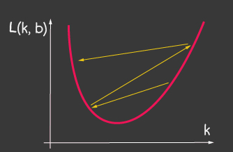
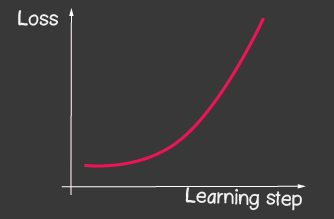
Where $\mu$ Is the learning rate and is one of the adjustable parameters of the model. For gradient descent, it does not change throughout the learning process. A small value of the learning rate can lead to a long convergence of the learning process of the model and a possible hit in the local minimum (Figure 2), and a very large value can lead to an infinite increase in the value of the error at each step of training, Figure 1.


Figure 1: The high value of the learning-rate	Figure 2: Small Learning-Rate

How to implement it without Tensorflow.js

For example, calculating the value of the loss function (standard deviation) would look like this:

function loss(ysPredicted, ysReal) {
    const squaredSum = ysPredicted.reduce(
        (sum, yPredicted, i) => sum + (yPredicted - ysReal[i]) ** 2,
        0);
    return squaredSum / ysPredicted.length;
}

However, the amount of input data can be large. During model training, we need to calculate not only the value of the loss function at each iteration, but also perform more serious operations - calculating the gradient. Therefore, it makes sense to use tensorflow, which optimizes calculations by using WebGL. Moreover, the code becomes much more expressive, compare:

    function loss(ysPredicted, ysReal) => {
        const ysPredictedTensor = tf.tensor(ysPredicted);
        const ysRealTensor = tf.tensor(ysReal);
        const loss = ysPredictedTensor.sub(ysRealTensor).square().mean();
        return loss.dataSync()[0];
    };

Solution with TensorFlow.js

The good news is that we will not have to write optimizers for a given error function (loss), we will not develop numerical methods for calculating partial derivatives, we have already implemented the backpropogation algorithm for us. We just need to follow these steps:

set a model (linear function, in our case);
describe the error function (in our case, this is the standard deviation)
choose one of the implemented optimizers (it is possible to extend the library with your own implementation)

What is tensor

Absolutely everyone has come across tensors in mathematics - these are scalar, vector, 2D - matrix, 3D - matrix. A tensor is a generalized concept of all of the above. This is a data container that contains data of a homogeneous type (tensorflow supports int32, float32, bool, complex64, string) and has a specific shape (the number of axes (rank) and the number of elements in each of the axes). Below we will consider tensors up to 3D matrices, but since this is a generalization, a tensor can have as many axes as we like: 5D, 6D, ... ND.

TensorFlow has the following API for tensor generation:

tf.tensor (values, shape?, dtype?)

where shape is the shape of the tensor and is given by an array, in which the number of elements is the number of axes, and each value of the array determines the number of elements along each of the axes. For example, to define a 4x2 matrix (4 rows, 2 columns), the form will take the form [4, 2].

Visualization	Description
	Scalar Rank: 0 Form: [] JS structure: `2` TensorFlow API: `tf.scalar(2); tf.tensor(2, []);`
	Vector Rank: 1 Shape: [4] JS structure: `[1, 2, 3, 4]` TensorFlow API: `tf.tensor([ 1, 2, 3, 4]); tf.tensor([1, 2, 3, 4], [4]); tf.tensor1d([1, 2, 3, 4]);`
	Matrix Rank: 2 Shape: [4,2] JS structure: `[ [1, 2], [3, 4], [5, 6], [7, 8] ]` TensorFlow API: `tf.tensor([[1, 2],[3, 4],[5,6],[7,8]]); tf.tensor([1, 2, 3, ... 7, 8], [4,2]); tf.tensor2d([[1, 2],[3, 4]...[7,8]]); tf.tensor2d([1, 2, 3, ... 7, 8], [4,2]);`
	Matrix Rank: 3 Shape: [4,2,3] JS structure: `[ [ [ 1, 2], [ 3, 4], [ 5, 6] ], [ [ 7, 8], [ 9, 10], [11, 12] ], [ [13, 14], [15, 16], [17, 18] ], [ [19, 20], [21, 22], [23, 24] ] ]` TensorFlow API: `tf.tensor([ [ [ 1, 2], [ 3, 4], [ 5, 6] ], .... [ [19, 20], [21, 22], [23, 24] ] ]); tf.tensor([1, 2, 3, .... 24], [4, 2 ,3])`

Linear approximation with TensorFlow.js

Initially, we'll talk about making the code extensible. We can transform the linear approximation into an approximation of the experimental points by a function of any kind. The class hierarchy will look like this:

Let's start implementing the methods of the abstract class, with the exception of the abstract methods that will be defined in the child classes, and here we will only leave stubs with errors if for some reason the method is not defined in the child class.

import * as tf from '@tensorflow/tfjs';

export default class AbstractRegressionModel {
    constructor(
        width,
        height,
        optimizerFunction = tf.train.sgd,
        maxEpochPerTrainSession = 100,
        learningRate = 0.1,
        expectedLoss = 0.001
    ) {
        this.width = width;
        this.height = height;
        this.optimizerFunction = optimizerFunction;
        this.expectedLoss = expectedLoss;
        this.learningRate = learningRate;
        this.maxEpochPerTrainSession = maxEpochPerTrainSession;

        this.initModelVariables();

        this.trainSession = 0;
        this.epochNumber = 0;
        this.history = [];
    }
}

So, in the constructor of the model we have defined width and height - these are the real width and height of the plane on which we will place the experimental points. This is necessary to normalize the input data. Those. if we have

x \in [0, w i d t h], y \in [0, h e i g h t]

$x\in[0, width], y\in[0, height]$ , then after normalization we will have:

x_{n o r m} \in [0, 1], y_{n o r m} \in [0, 1]

$x_{norm}\in[0, 1], y_{norm}\in[0, 1]$

optimizerFunction - we will make the task of the optimizer flexible, in order to be able to try other optimizers available in the library, by default we have set the Stochastic Gradient Descent method tf.train.sgd . I would also recommend playing with other available optimizers that can tweak the learningRate during training and the learning process is greatly improved, for example, try the following optimizers: tf.train.momentum , tf.train.adam .

In order for the learning process not to endlessly, we have defined two parameters maxEpochPerTrainSesion and expectedLoss- in this way we will stop the training process either when the maximum number of training iterations is reached, or when the value of the error function becomes lower than the expected error (we will take everything into account in the train method below).

In the constructor, we call the initModelVariables method - but as agreed, we stub and define it in the child class later.

initModelVariables() {
    throw Error('Model variables should be defined')
}

Now let's implement the main method of the train model:

/**
     * Train model until explicitly stop process via invocation of stop method
     * or loss achieve necessary accuracy, or train achieve max epoch value
     *
     * @param x - array of x coordinates
     * @param y - array of y coordinates
     * @param callback - optional, invoked after each training step
     */
    async train(x, y, callback) {
        const currentTrainSession = ++this.trainSession;
        this.lossVal = Number.POSITIVE_INFINITY;
        this.epochNumber = 0;
        this.history = [];

        // convert array into tensors
        const input = tf.tensor1d(this.xNormalization(x));
        const output = tf.tensor1d(this.yNormalization(y));

        while (
            currentTrainSession === this.trainSession
            && this.lossVal > this.expectedLoss
            && this.epochNumber <= this.maxEpochPerTrainSession
            ) {
            const optimizer = this.optimizerFunction(this.learningRate);
            optimizer.minimize(() => this.loss(this.f(input), output));
            this.history = [...this.history, {
                epoch: this.epochNumber,
                loss: this.lossVal
            }];
            callback && callback();
            this.epochNumber++;
            await tf.nextFrame();
        }
    }

trainSession is essentially a unique identifier for the training session in case the external API calls the train method, while the previous training session has not ended yet.

From the code you can see that we create tensor1d from one-dimensional arrays, while the data must be normalized beforehand, the functions for normalization are here:

xNormalization = xs => xs.map(x => x / this.width);
yNormalization = ys => ys.map(y => y / this.height);
yDenormalization = ys => ys.map(y => y * this.height);

In a loop, for each training step, we call the model optimizer, to which we need to pass the loss function. As agreed, the loss function will be set by the standard deviation. Then using the API tensorflow.js we have:

    /**
     * Calculate loss function as mean-square deviation
     *
     * @param predictedValue - tensor1d - predicted values of calculated model
     * @param realValue - tensor1d - real value of experimental points
     */
    loss = (predictedValue, realValue) => {
        // L = sum ((x_pred_i - x_real_i)^2) / N
        const loss = predictedValue.sub(realValue).square().mean();
        this.lossVal = loss.dataSync()[0];
        return loss;
    };

The learning process continues while

the limit on the number of iterations will not be reached
the desired error accuracy will not be achieved
a new training process has not started

Also notice how the loss function is called. To get predictedValue - we call the function f - which, in fact, will set the form according to which the regression will be performed, and in the abstract class, as agreed, we put a stub:

  f(x) {
        throw Error('Model should be defined')
  }

At each step of training, in the property of the object of the history model, we save the dynamics of the error change at each training epoch.

After the process of training the model, we need to have a method that accepts inputs and outputs the calculated outputs using the trained model. To do this, in the API, we have defined the predict method and it looks like this:

/**
     * Predict value basing on trained model
     *  @param x - array of x coordinates
     *  @return Array({x: integer, y: integer}) - predicted values associated with input
     *
     * */
    predict(x) {
        const input = tf.tensor1d(this.xNormalization(x));
        const output = this.yDenormalization(this.f(input).arraySync());
        return output.map((y, i) => ({ x: x[i], y }));
    }

Pay attention to arraySync , by analogy with node.js, if there is an arraySync method, then there is definitely an asynchronous array method that returns a Promise. Promise is needed here, because as we said earlier, tensors are all migrated to WebGL to speed up calculations and the process becomes asynchronous, because it takes time to move data from WebGL to a JS variable.

We are done with an abstract class, you can see the full version of the code here:

AbstractRegressionModel.js

import * as tf from '@tensorflow/tfjs';

export default class AbstractRegressionModel {
    
    constructor(
        width,
        height,
        optimizerFunction = tf.train.sgd,
        maxEpochPerTrainSession = 100,
        learningRate = 0.1,
        expectedLoss = 0.001
    ) {
        this.width = width;
        this.height = height;
        this.optimizerFunction = optimizerFunction;
        this.expectedLoss = expectedLoss;
        this.learningRate = learningRate;
        this.maxEpochPerTrainSession = maxEpochPerTrainSession;

        this.initModelVariables();

        this.trainSession = 0;
        this.epochNumber = 0;
        this.history = [];
    }

    initModelVariables() {
        throw Error('Model variables should be defined')
    }

    f() {
        throw Error('Model should be defined')
    }

    xNormalization = xs => xs.map(x => x / this.width);
    yNormalization = ys => ys.map(y => y / this.height);
    yDenormalization = ys => ys.map(y => y * this.height);

    /**
     * Calculate loss function as mean-squared deviation
     *
     * @param predictedValue - tensor1d - predicted values of calculated model
     * @param realValue - tensor1d - real value of experimental points
     */
    loss = (predictedValue, realValue) => {
        const loss = predictedValue.sub(realValue).square().mean();
        this.lossVal = loss.dataSync()[0];
        return loss;
    };

    /**
     * Train model until explicitly stop process via invocation of stop method
     * or loss achieve necessary accuracy, or train achieve max epoch value
     *
     * @param x - array of x coordinates
     * @param y - array of y coordinates
     * @param callback - optional, invoked after each training step
     */
    async train(x, y, callback) {
        const currentTrainSession = ++this.trainSession;
        this.lossVal = Number.POSITIVE_INFINITY;
        this.epochNumber = 0;
        this.history = [];

        // convert data into tensors
        const input = tf.tensor1d(this.xNormalization(x));
        const output = tf.tensor1d(this.yNormalization(y));

        while (
            currentTrainSession === this.trainSession
            && this.lossVal > this.expectedLoss
            && this.epochNumber <= this.maxEpochPerTrainSession
            ) {
            const optimizer = this.optimizerFunction(this.learningRate);
            optimizer.minimize(() => this.loss(this.f(input), output));
            this.history = [...this.history, {
                epoch: this.epochNumber,
                loss: this.lossVal
            }];
            callback && callback();
            this.epochNumber++;
            await tf.nextFrame();
        }
    }

    stop() {
        this.trainSession++;
    }

    /**
     * Predict value basing on trained model
     *  @param x - array of x coordinates
     *  @return Array({x: integer, y: integer}) - predicted values associated with input
     *
     * */
    predict(x) {
        const input = tf.tensor1d(this.xNormalization(x));
        const output = this.yDenormalization(this.f(input).arraySync());
        return output.map((y, i) => ({ x: x[i], y }));
    }
}

For linear regression, we define a new class that will inherit from the abstract class, where we only need to define two methods initModelVariables and f .

Since we are working on a linear approximation, we must specify two variables k, b - and they will be scalar tensors. For the optimizer, we must indicate that they are customizable (variables), and assign arbitrary numbers as initial values.

initModelVariables() {
   this.k = tf.scalar(Math.random()).variable();
   this.b = tf.scalar(Math.random()).variable();
}

Consider the API for variable here :

tf.variable (initialValue, trainable?, name?, dtype?)

Pay attention to the second argument to trainable - a boolean variable and by default it is true . It is used by optimizers, which tells them whether it is necessary to configure this variable when minimizing the loss function. This can be useful when we are building a new model based on a pretrained model downloaded from Keras Python, and we are sure that there is no need to retrain some layers in this model.

Next, we need to define the equation of the approximating function using tensorflow API, take a look at the code and you will intuitively understand how to use it:

f(x) {
   // y = kx + b
   return  x.mul(this.k).add(this.b);
}

For example, this way you can define a quadratic approximation:

initModelVariables() {
   this.a = tf.scalar(Math.random()).variable();
   this.b = tf.scalar(Math.random()).variable();
   this.c = tf.scalar(Math.random()).variable();
}

f(x) {
    // y = ax^2 + bx + c
    return this.a.mul(x.square()).add(this.b.mul(x)).add(this.c);
}

Here you can check out the models for linear and quadratic regression:

LinearRegressionModel.js

import * as tf from '@tensorflow/tfjs';
import AbstractRegressionModel from "./AbstractRegressionModel";

export default class LinearRegressionModel extends AbstractRegressionModel {
    initModelVariables() {
        this.k = tf.scalar(Math.random()).variable();
        this.b = tf.scalar(Math.random()).variable();
    }

    f = x => x.mul(this.k).add(this.b);
}

QuadraticRegressionModel.js

import * as tf from '@tensorflow/tfjs';
import AbstractRegressionModel from "./AbstractRegressionModel";

export default class QuadraticRegressionModel extends AbstractRegressionModel {
    initModelVariables() {
        this.a = tf.scalar(Math.random()).variable();
        this.b = tf.scalar(Math.random()).variable();
        this.c = tf.scalar(Math.random()).variable();
    }

    f = x => this.a.mul(x.square()).add(this.b.mul(x)).add(this.c);
}

Below is some code written in React that uses the written linear regression model and creates the UX for the user:

Regression.js

import React, { useState, useEffect } from 'react';

import Canvas from './components/Canvas';
import LossPlot from './components/LossPlot_v3';
import LinearRegressionModel from './model/LinearRegressionModel';

import './RegressionModel.scss';

const WIDTH = 400;
const HEIGHT = 400;
const LINE_POINT_STEP = 5;

const predictedInput = Array.from({ length: WIDTH / LINE_POINT_STEP + 1 })
    .map((v, i) => i * LINE_POINT_STEP);

const model = new LinearRegressionModel(WIDTH, HEIGHT);

export default () => {
    const [points, changePoints] = useState([]);
    const [curvePoints, changeCurvePoints] = useState([]);
    const [lossHistory, changeLossHistory] = useState([]);

    useEffect(() => {
        if (points.length > 0) {
            const input = points.map(({ x }) => x);
            const output = points.map(({ y }) => y);

            model.train(input, output, () => {
                changeCurvePoints(() => model.predict(predictedInput));
                changeLossHistory(() => model.history);
            });
        }
    }, [points]);

    return (
        <div className="regression-low-level">
            <div className="regression-low-level__top">
                <div className="regression-low-level__workarea">
                    <div className="regression-low-level__canvas">
                        <Canvas
                            width={WIDTH}
                            height={HEIGHT}
                            points={points}
                            curvePoints={curvePoints}
                            changePoints={changePoints}
                        />
                    </div>
                    <div className="regression-low-level__toolbar">
                        <button
                            className="btn btn-red"
                            onClick={() => model.stop()}>Stop
                        </button>
                        <button
                            className="btn btn-yellow"
                            onClick={() => {
                                model.stop();
                                changePoints(() => []);
                                changeCurvePoints(() => []);
                            }}>Clear
                        </button>
                    </div>
                </div>
                <div className="regression-low-level__loss">
                    <LossPlot
                              loss={lossHistory}/>
                </div>

            </div>
        </div>
    )
}

Result:

I would highly recommend doing the following tasks:

to implement the function approximation by the logarithmic function
for the tf.train.sgd optimizer, try playing with learningRate and watching the learning process change. Try to set the learningRate very high to get the picture shown in Figure 2.
set the optimizer to tf.train.adam. Has the learning process improved? Whether the learning process depends on changing the learningRate value in the model constructor.

TensorFlow.js: Part 1: Using the Low-Level API to Approximate Linear Functions