Book "Natural Language Processing in Action"

Hello Habitants! We have published a practical guide to processing and generating natural language texts. The book is equipped with all the tools and techniques necessary to create applied NLP systems in order to ensure the operation of a virtual assistant (chat bot), a spam filter, a forum moderator program, a sentiment analyzer, a knowledge base building program, an intelligent natural language text analyzer, or just about any other NLP application you can imagine.



The book is aimed at intermediate to advanced Python developers. A significant part of the book will be useful to those readers who already know how to design and develop complex systems, as it contains numerous examples of recommended solutions and reveals the capabilities of the most modern NLP algorithms. While knowledge of object-oriented programming in Python can help you build better systems, it is not required to use the information in this book.

Feedback neural networks: recurrent neural networks

Chapter 7 demonstrates the possibilities of analyzing a fragment or a whole sentence using a convolutional neural network, tracking adjacent words in a sentence by applying a shared weights filter (performing convolution) on them. Words occurring in groups can also be found in a bundle. The web is also resistant to small shifts in the positions of these words. At the same time, adjacent concepts can significantly affect the network. But if you need to take a look at the big picture of what is happening, take into account the relationships over a longer period of time, a window covering more than 3-4 tokens from the supply? How to introduce the concept of past events into the network? Memory?



For each training example (or batch of disordered examples) and output (or batch of outputs) of the feed forward neural network, the weights of the neural network need to be adjusted for individual neurons based on the backpropagation method. We have already demonstrated this. But the results of the training phase for the following example are mostly independent of the order of the input data. Convolutional neural networks seek to capture these order relationships by capturing local relationships, but there is another way.



In a convolutional neural network, each training example is passed to the network as a grouped set of word tokens. The word vectors are grouped into a matrix in the form (length of the word vector × number of words in the example), as shown in Fig. 8.1.





But this sequence of word vectors can be just as easily conveyed to the normal feedforward neural network from Chapter 5 (Figure 8.2), right?





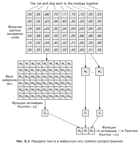
Of course, this is a perfectly workable model. With this method of passing input data, the feedforward neural network will be able to respond to joint occurrences of tokens, which is what we need. But at the same time, it will react to all joint occurrences in the same way, regardless of whether they are separated by a long text, or they are next to each other. In addition, feedforward neural networks, like CNNs, are poor at handling variable-length documents. They are unable to process text at the end of the document if it goes beyond the width of the web.



Feedforward neural networks perform best in modeling the relationship of a data sample as a whole with its corresponding label. Words at the beginning and at the end of a sentence have the same effect on the output signal as in the middle, despite the fact that they are unlikely to be semantically related to each other.



This uniformity (uniformity of influence) can clearly cause problems in the case of, for example, harsh negation tokens and modifiers (adjectives and adverbs) such as "no" or "good". In a feedforward neural network, negation words affect the meaning of all words in a sentence, even if they are far removed from the place they should actually influence.



One-dimensional convolutions is a way to solve these relationships between tokens by parsing multiple words across windows. The downsampling layers discussed in Chapter 7 are specifically designed to accommodate small word order changes. In this chapter, we'll look at another approach that will help us take the first step towards the concept of neural network memory. Instead of disassembling a language as a large chunk of data, we'll start looking at its sequential formation, token by token, over time.

8.1. Memorization in neural networks

Of course, words in a sentence are rarely completely independent of each other; their occurrences are influenced or influenced by occurrences of other words in the document. For example: The stolen car sped into the arena and The clown car sped into the arena.



You may have completely different impressions of the two sentences when you read to the end. The construction of the phrase in them is the same: adjective, noun, verb and prepositional phrase. But replacing the adjective in them radically changes the essence of what is happening from the point of view of the reader.



How to simulate such a relationship? How to understand that arena and even sped can have slightly different connotations if there is an adjective in front of them in the sentence that is not a direct definition of any of them?



If there was a way to remember what happened a moment earlier (especially remember what happened at step t at step t + 1), it would be possible to identify patterns that arise when certain tokens appear in a sequence of patterns associated with other tokens. Recurrent neural networks (RNNs) make it possible for a neural network to memorize the past words of a sequence.



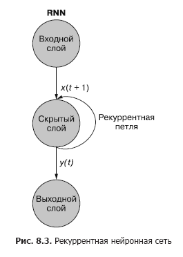
As you can see in fig. 8.3, a separate recurrent neuron from the hidden layer adds a recurrent loop to the network to "reuse" the output of the hidden layer at time t. The output at time t is added to the next input at time t + 1. The network processes this new input at time step t + 1 to produce a hidden layer output at time t + 1. This output at time t + 1 then it is reused by the network and included in the input signal at a time step t + 2, etc.





While the idea of ​​influencing a state through time looks a little confusing, the basic concept is simple. The results of each signal at the input of a conventional feedforward neural network at a time step t are used as an additional input signal along with the next piece of data fed to the network input at a time step t + 1. The network receives information not only about what is happening now, but also about what happened before ...

. , . , . , . , . , , . . , .



t . , t = 0 — , t + 1 — . () . , . — .



t, — t + 1.

A recurrent neural network can be visualized as shown in Fig. 8.3: The circles correspond to entire layers of a feedforward neural network, consisting of one or more neurons. The output of the hidden layer is issued by the network as usual, but then comes back as its own (hidden layer) input along with the usual input data of the next time step. The diagram depicts this feedback loop as an arc leading from the output of the layer back to the input.



An easier (and more commonly used) way to illustrate this process is using network deployment. Figure 8.4 shows an upside-down network with two sweeps of the time variable (t) - layers for steps t + 1 and t + 2.





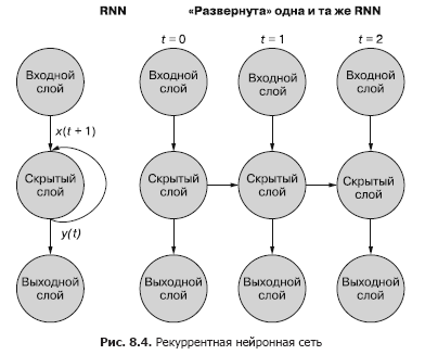
Each of the time steps corresponds to an expanded version of the same neural network in the form of a column of neurons. It's like watching a script or individual video frames of a neural network at any given time. The net on the right represents a future version of the net on the left. The output signal of the hidden layer at time (t) is fed back to the input of the hidden layer along with the input data for the next time step (t + 1) on the right. Once again. The diagram shows two iterations of this deployment, a total of three columns of neurons for t = 0, t = 1, and t = 2.



All vertical routes in this diagram are completely analogous, they show the same neurons. They reflect the same neural network at different points in time. This visualization is useful for demonstrating the forward and backward movement of information over the network during back propagation of an error. But remember when looking at these three networks deployed: they are different snapshots of the same network with the same set of weights.



Let's take a closer look at the original representation of the recurrent neural network before deploying it and show the relationship between the input signals and weights. The individual layers of this RNN look as shown in Fig. 8.5 and 8.6.





All latent state neurons have a set of weights applied to each of the elements of each of the input vectors, as in a conventional feedforward network. But in this scheme, an additional set of trainable weights appeared, which are applied to the output signals of hidden neurons from the previous time step. The network, by training, selects the appropriate weights (importance) of previous events when entering the sequence token by token.

«», t = 0 t – 1. «» , , . t = 0 . , .

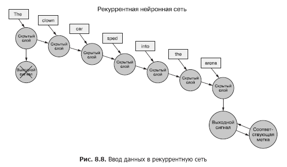
Back to the data, imagine you have a set of documents, each of which is a labeled example. And instead of transferring the entire set of word vectors to the convolutional neural network for each sample, as in the previous chapter (Figure 8.7), we transfer the sample data to the RNN, one token at a time (Figure 8.8).





We pass in a vector of words for the first token and get the output of our recurrent neural network. Then we transfer the second token, and with it the output signal from the first! After that, we transfer the third token along with the output signal from the second! Etc. Now in our neural network there are concepts of "before" and "after", cause and effect, some, albeit vague, notion of time (see Fig. 8.8).





Now our network is already remembering something! Well, to a certain extent. There are still a few things left to figure out. First, how can back propagation of an error occur in such a structure?

8.1.1. Back propagation of an error in time

All of the networks discussed above have had the target label (target variable), and RNN is no exception. But we do not have the concept of a label for each token, and there is only one label for all tokens of each of the sample text. We only have labels for sample documents.

We are talking about tokens as input to the network at each time step, but recurrent neural networks can also work with any time series data. Tokens can be any, discrete or continuous: weather station readings, notes, symbols in a sentence, etc.

Here we first compare the output of the network at the last time step with the cue. This is what we will (for now) call an error, namely, our network is trying to minimize it. But there is a slight difference from the previous chapters. A given sample of data is split into smaller pieces that are fed into the neural network sequentially. However, instead of directly using the output for each of these sub-examples, we send it back to the network.



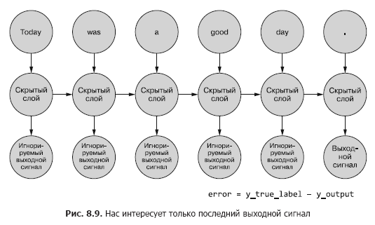
So far, we are only interested in the final output signal. Each of the tokens in the sequence is fed into the network, and losses are calculated based on the output of the last time step (token) (Figure 8.9).





It is necessary to determine, if there is an error for a given example, which weights to update and how much. In Chapter 5, we showed you how to backpropagate an error over a normal network. And we know that the amount of weight correction depends on its (this weight) contribution to the error. We can feed a token from a sample sequence to the input of the network, calculating the error for the previous time step based on its output signal. This is where the idea of ​​backpropagating an error in time seems to confuse everything.



However, one can simply think of it as a time-bound process. At each time step, tokens, starting from the first at t = 0, are fed one at a time to the input of the hidden neuron located in front - the next column in Fig. 8.9. At the same time, the network expands, revealing the next column of the network, already ready to receive the next token in the sequence. Latent neurons unfold one at a time, like a music box or a mechanical piano. In the end, when all the elements of the examples are fed into the network, there will be nothing more to deploy and we will get a final label for the target variable of interest to us, which can be used to calculate the error and adjust the weights. We've just gone all the way down the compute graph for this unrolled net.



For now, we consider the input data to be generally static. You can trace through the entire graph which input signal enters which neuron. And since we know how which neuron works, we can propagate the error back along the chain, along the same path, just like in the case of a conventional feedforward neural network.



To propagate the error back to the previous layer, we will use the chain rule. Instead of the previous layer, we will propagate the error to the same layer in the past, as if all the deployed network variants were different (Figure 8.10). This does not change the calculation mathematics.





The error propagates back from the last step. The gradient of an earlier time step relative to a newer one is calculated. After calculating all individual token-based gradients up to step t = 0 for this example, the changes are aggregated and applied to one set of weights.

8.1.2. When to update what

We've turned our weird RNN into something like a regular feedforward neural network, so updating the weights shouldn't be too difficult. However, there is one caveat. The trick is that the weights are not updated in another branch of the neural network at all. Each branch represents the same network at different points in time. The weights for each time step are the same (see Figure 8.10).



A simple solution to this problem is to calculate corrections for the weights at each of the time steps with a delay in the update. In a feedforward network, all updates to the weights are computed immediately after computation of all gradients for a particular input signal. And here it is exactly the same, but updates are deferred until we get to the initial (zero) time step for a specific input sample data.



The calculation of the gradient should be based on the values ​​of the weights at which they made this contribution to the error. Here's the most overwhelming part: the weight at time step t contributed in some way to the error. And the same weight receives a different input signal at the time step t + 1, which means that it makes a different contribution to the error.



You can compute the various changes in the weights at each time step, sum them up, and then apply the grouped changes to the weights of the hidden layer as the last step in the training phase.

, . , , . , , . , .

Real magic. In the case of backward propagation of the error in time, an individual weight can be corrected in one direction at a time step t (depending on its response to the input signal at a time step t), and then in the other direction at a time step t - 1 (in accordance with how it reacted to the input signal at time step t - 1) for one data sample! Remember that neural networks in general are based on minimizing the loss function regardless of the complexity of the intermediate steps. Collectively, the network optimizes this complex feature. Since the weight update is applied only once for the example data, the network (if it converges at all, of course) eventually stops at the most optimal weight in this sense for a specific input signal and a specific neuron.

The results of the previous steps are still important

Sometimes the whole sequence of values ​​generated at all intermediate time steps is important. In Chapter 9, we'll give examples of situations in which the output of a particular time step t is just as important as the output of the last time step. In fig. 8.11 shows a method for collecting error data for any time step and propagating it back to correct all network weights.





This process resembles the usual back propagation of an error in time for n time steps. In this case, we propagate the bug back from several sources at the same time. But, as in the first example, the weight adjustments are additive. The error propagates from the last time step at the beginning to the first with the sum of the changes in each of the weights. Then the same thing happens with the error computed at the penultimate time step, summing all changes up to t = 0. This process is repeated until we reach time step zero with back propagation of the error for it as if it were the only one. Then the cumulative changes are applied all at once to the corresponding hidden layer.



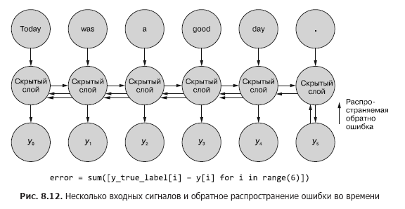
In fig. Figure 8.12 shows how the error propagates from each output signal back to t = 0, then is aggregated before the final correction of the weights. This is the main idea of ​​this section. As in the case of a conventional feedforward neural network, the weights are updated only after calculating the proposed change in weights for the entire backpropagation step for a given input signal (or set of input signals). In the case of RNN, the back propagation of the error includes updates up to time t = 0.



Updating the weights earlier would have skewed the gradient calculations with back propagation errors at earlier points in time. Remember, gradients are calculated relative to a specific weight. If this weight is updated too early, say at time step t, then when calculating the gradient at time step t - 1, the weight value (recall that this is the same position of the weight in the network) will change. And when calculating the gradient based on the input signal from the time step t - 1, the calculations will be distorted. In fact, in this case, the weight will be fined (or rewarded) for what is "not to blame"!

About the authors

Hobson Lane(Hobson Lane) has 20 years of experience building autonomous systems that make critical decisions for the benefit of people. At Talentpair, Hobson taught machines to read and understand résumés in a less biased manner than most hiring managers. At Aira, he helped build their first chatbot designed to interpret the world around the blind. Hobson is a passionate admirer of AI's openness and community-driven orientation. He makes active contributions to open source projects such as Keras, scikit-learn, PyBrain, PUGNLP, and ChatterBot. He is currently involved in open research and educational projects for Total Good, including creating an open source virtual assistant. He has published numerous articles, has lectured at AIAA, PyCon,PAIS and IEEE and has received several patents in the field of robotics and automation.



Hannes Max Hapke is an electrical engineer turned machine learning engineer. In high school, he became interested in neural networks when he studied ways to compute neural networks on microcontrollers. Later in college, he applied the principles of neural networks to the efficient management of renewable energy power plants. Hannes is passionate about automating software development and machine learning pipelines. He has co-authored deep learning models and machine learning pipelines for the recruiting, energy and healthcare industries. Hannes has given presentations on machine learning at a variety of conferences including OSCON, Open Source Bridge and Hack University.



Cole Howard(Cole Howard) is a machine learning practitioner, NLP practitioner and writer. An eternal seeker of patterns, he found himself in the world of artificial neural networks. Among his developments are large-scale recommendation systems for trading over the Internet and advanced neural networks for ultra-high-dimensional machine intelligence systems (deep neural networks), which take first places in the Kaggle competitions. He has given talks on convolutional neural networks, recurrent neural networks, and their role in natural language processing at the Open Source Bridge and Hack University conferences.





»More details about the book can be found on the website of the publishing house

» Table of Contents

» Excerpt



For Habitants a 25% discount on coupon - NLP



Upon payment for the paper version of the book, an e-book is sent to the e-mail.