🍻 🤶🏽 🧔🏼 Move an object evenly along a curve 🍂 🙌🏿 👨🏻‍🌾

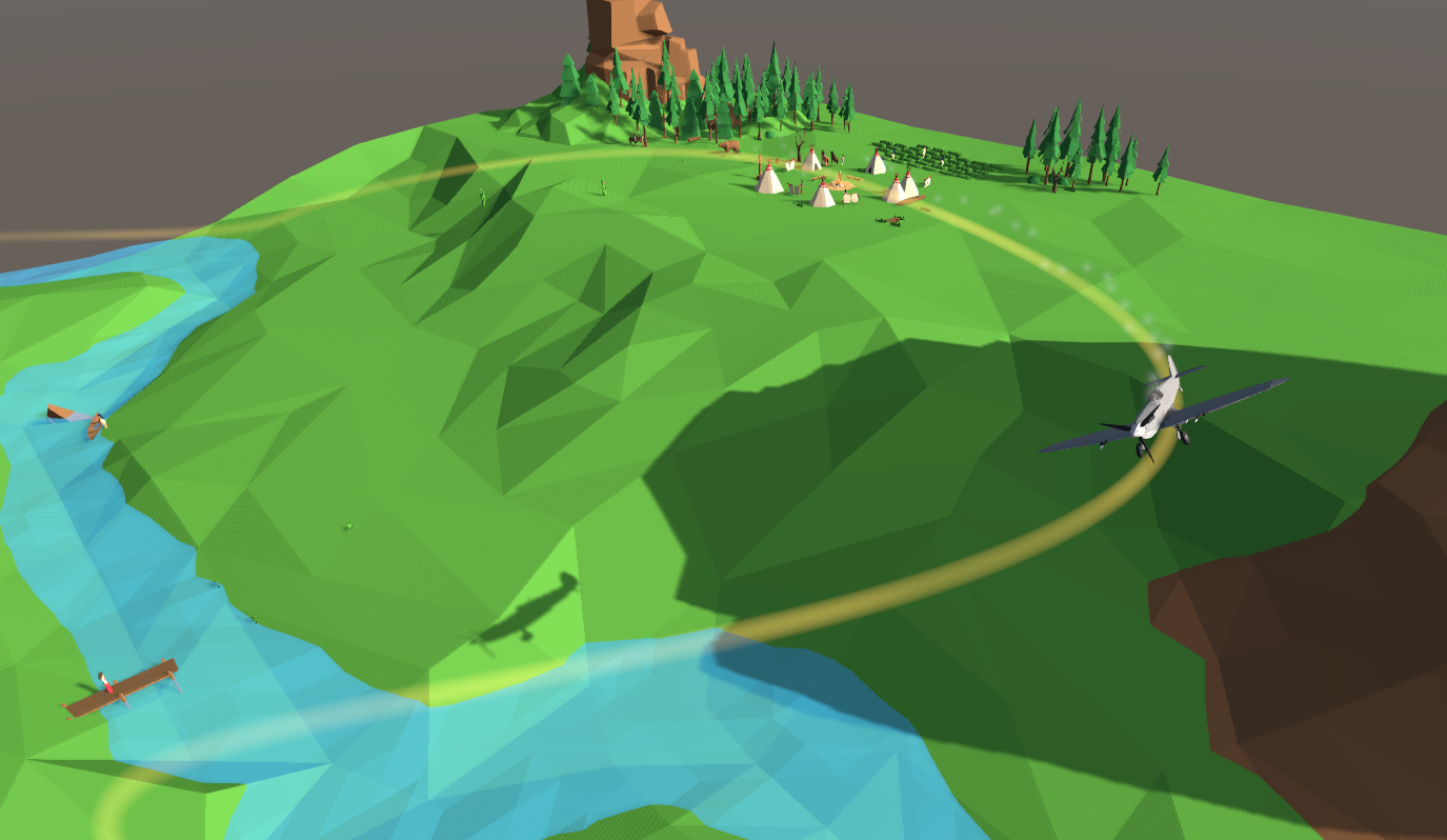
In the process of developing a game in completely different genre categories, it may be necessary to "launch" any game object along a smooth curve at a constant or controlled speed, be it a truck moving from city A to city B, a missile fired along a cunning trajectory, or an enemy plane performing a laid down maneuver.

Probably, everyone related to the topic knows or at least heard about Bézier curves, B-splines, Hermite splines and other interpolation and smoothing splines and would absolutely correctly suggest using one of them in the described situation, but not everything is so simple as we would like.

In our case, a spline is a function that displays a set of input parameters (control points) and the value of an argument

t

$t$ (usually taking values from 0 to 1) to a point on a plane or in space. The resulting curve is the set of values of the spline function for

t \in [0, 1]

$t\in[0,1]$ .

As an example, consider the cubicBezier curve, which is given by the following equation:

Cubic Bezier Curve

The figure shows two cubic Bezier curves, specified by four points (the curve passes through two of them, the remaining two define the curvature).

Animation of displaying the parameter t to a curve point

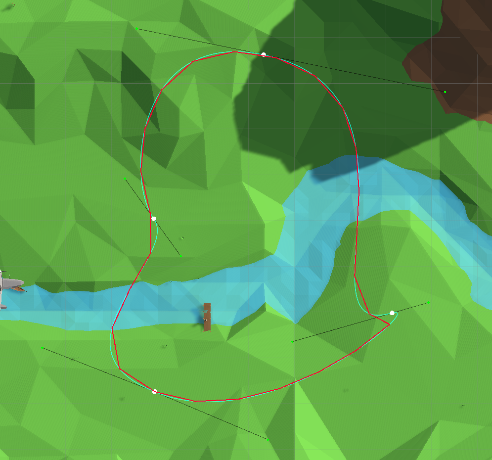
In order to build a more complex and variable route from the curve sections, they can be connected in a chain, leaving one common point-link:

Piecewise spline We have

figured out the task and parameterization of the route, now we turn to the main question. In order for our conditional plane to move along the route at a constant speed, we need at any time to be able to calculate a point on the curve, depending on the distance traveled along this curve.

s (l e n)

$s(len)$ , while having only the ability to calculate the position of a point on the curve from the value of the parameter

t

$t$ (function

y (t)

$y(t)$ ). It is at this stage that difficulties begin.

My first thought was to do a linear mapping

l e n \in [0, L e n g t h] \Rightarrow t \in [0, 1]

$len\in[0, Length] \Rightarrow t\in[0,1]$ and calculate

y (t)

$y(t)$ from the resulting value - easy, computationally cheap, in general, what you need.

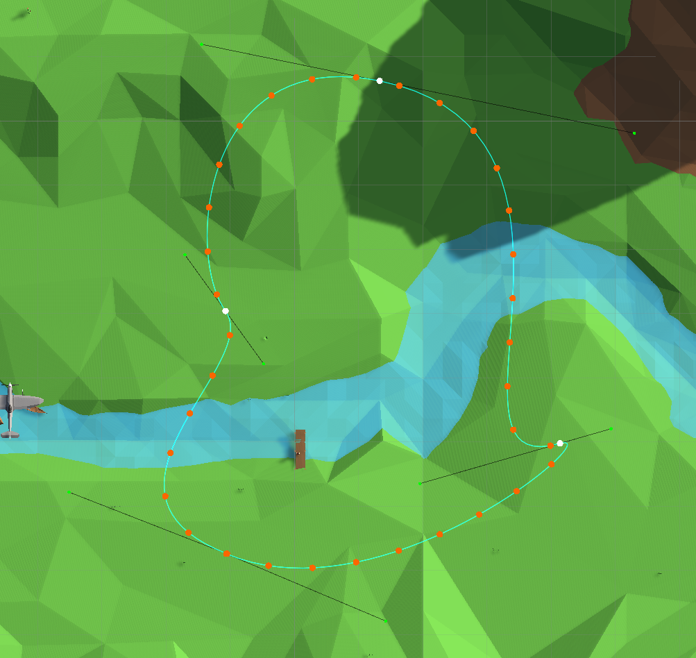
The problem with this method is immediately obvious - in fact, the distance covered

s

$s$ depends on

t

$t$ nonlinear, and in order to be convinced of this, it is enough to arrange along the route uniformly distributed

t

$t$ points:

“evenly” distributed points along the path

The plane will slow down in some sections and accelerate in others, which makes this method of parameterization of the curve completely inapplicable for solving the described problem was pursued):

Visualizing the wrong parameterization of the curve

After consulting the search engine, onstackoverflowandyoutube, I discovered a second way to calculate

s (l e n) = g (t)

$s(len) = g(t)$ , namely the representation of the curve in the form of a piecewise linear function (calculating a set of points equidistant from each other along the curve):

Representing the curve in the form of a piecewise linear spline

This procedure is iterative: a small step is taken

t

$t$ , we move along a curve with it, summing the distance traveled as the length of a piecewise linear spline until the specified distance is covered, after which the point is remembered, and the process resumes.

Sample code

A source

public Vector2[] CalculateEvenlySpacedPoints(float spacing, float resolution = 1)
  {
    List<Vector2> evenlySpacedPoints = new List<Vector2>();
    evenlySpacedPoints.Add(points[0]);
    Vector2 previousPoint = points[0];
    float dstSinceLastEvenPoint = 0;

    for (int segmentIndex = 0; segmentIndex < NumSegments; segmentIndex++)
    {
      Vector2[] p = GetPointsInSegment(segmentIndex);
      float controlNetLength = Vector2.Distance(p[0], p[1]) + Vector2.Distance(p[1], p[2]) + Vector2.Distance(p[2], p[3]);
      float estimatedCurveLength = Vector2.Distance(p[0], p[3]) + controlNetLength / 2f;
      int divisions = Mathf.CeilToInt(estimatedCurveLength * resolution * 10);
      float t = 0;
      while (t <= 1)
      {
        t += 1f/divisions;
        Vector2 pointOnCurve = Bezier.EvaluateCubic(p[0], p[1], p[2], p[3], t);
        dstSinceLastEvenPoint += Vector2.Distance(previousPoint, pointOnCurve);

        while (dstSinceLastEvenPoint >= spacing)
        {
          float overshootDst = dstSinceLastEvenPoint - spacing;
          Vector2 newEvenlySpacedPoint = pointOnCurve + (previousPoint - pointOnCurve).normalized * overshootDst;
          evenlySpacedPoints.Add(newEvenlySpacedPoint);
          dstSinceLastEvenPoint = overshootDst;
          previousPoint = newEvenlySpacedPoint;
        }

        previousPoint = pointOnCurve;
      }
    }

    return evenlySpacedPoints.ToArray();
  }

And, it seems, the task is solved, because you can split the route into many segments and enjoy how smoothly and measuredly the object moves, since calculating a point on a piecewise linear function is a simple and fast matter. But this approach also has quite obvious drawbacks that bothered me - a rather costly procedure for changing the partition step or curve geometry and the need to find a balance between accuracy (more memory consumption) and memory savings (the "broken" route becomes more noticeable).

As a result, I continued my search and came across an excellent article "Moving Along a Curve with Specified Speed" , on the basis of which further reasoning is based.

The speed value can be calculated as

σ (t) = | V (t) | = | \frac{d X}{d t} |

$\sigma(t) = |V(t)|=|\frac{dX}{dt}|$ where

X (t)

$X(t)$ is a spline function. To solve the problem, you need to find the function

Y (t) = X (s)

$Y(t)=X(s)$ , where

s

$s$ - the length of the arc from the starting point to the desired one, and this expression sets the relationship between

t

$t$ and

s

$s$ .

Using differentiation variable substitution, we can write

\frac{d Y}{d t} = \frac{d X}{d s} \frac{d s}{d t} .

$\frac{dY}{dt}=\frac{dX}{ds}\frac{ds}{dt}.$

Taking into account that the velocity is a non-negative quantity, we obtain

| \frac{d Y}{d t} | = | \frac{d X}{d s} | | \frac{d s}{d t} | = \frac{d s}{d t},

$|\frac{dY}{dt}|=|\frac{dX}{ds}||\frac{ds}{dt}|=\frac{ds}{dt},$

because

| \frac{d X}{d s} | = 1

$|\frac{dX}{ds}| = 1$ by the condition that the modulus of the velocity vector remains unchanged (generally speaking,

| \frac{d X}{d s} |

$|\frac{dX}{ds}|$ is not equal to one, but to a constant, but for simplicity of calculations we will take this constant equal to one).

Now we get the ratio between

t

$t$ and

s

$s$ explicitly:

s = g (t) = \int_{0}^{t} | \frac{d Y (τ)}{d t} | d τ,

$s=g(t)=\int_{0}^{t}|\frac{dY(\tau)}{dt}|d\tau,$

whence the total length of the curve

L

$L$ is obviously calculated as

g (1)

$g(1)$ . Using the resulting formula, it is possible, having the value of the argument

t

$t$ , compute the length of the arc to the point at which this value is

t

$t$ displayed.

We are interested in the reverse operation, that is, calculating the value of the argument

t

$t$ along a given arc length

s

$s$ :

t = g^{- 1} (s) .

$t=g^{-1}(s).$

Since there is no general analytical way to find the inverse function, you will have to look for a numerical solution. We denote

F (t) = g (t) - s .

$F(t)=g(t)-s.$ For a given

s

$s$ , you need to find such a value

t

$t$ at which

F (t) = 0

$F(t)=0$ . Thus, the task turned into the task of finding the root of the equation, which Newton's method can perfectly cope with.

The method forms a sequence of approximations of the form

t_{i + 1} = t_{i} - \frac{F (t_{i})}{F^{'} (t_{i})},

$t_{i+1}=t_i-\frac{F(t_i)}{F'(t_i)},$

Where

F^{'} (t) = \frac{d F}{d t} = \frac{d g}{d t} = | \frac{d Y}{d t} | .

$F'(t)=\frac{dF}{dt}=\frac{dg}{dt}=|\frac{dY}{dt}|.$

To calculate

F (t)

$F(t)$ is required to calculate

g (t)

$g(t)$ , the calculation of which, in turn, requires numerical integration.

Choice

t_{0} = \frac{s}{L}

$t_0=\frac{s}{L}$ as an initial approximation now looks reasonable (recall the first approach to solving the problem).

Next, we iterate using Newton's method until the solution error becomes acceptable, or the number of iterations done is prohibitively large.

There is a potential problem with using Newton's standard method. Function

F (t)

$F(t)$ is non-decreasing, since its derivative

F^{'} (t) = | d Y / d t |

$F'(t)=|dY/dt|$ is non-negative. If the second derivative

F^{″} (t) > 0

$F''(t)>0$

F^{″} (t)

$F''(t)$ may turn out to be negative, due to which Newton's method may converge outside the definition range

t \in [0, 1]

$t\in[0,1]$ ... The author of the article proposes to use a modification of Newton's method, which, if the next iteration result by Newton's method does not fall into the current interval bounding the root, instead selects the middle of the interval ( dichotomy method ). Regardless of the result of the calculation at the current iteration, the range is narrowed, which means that the method converges to the root.

It remains to choose the method of numerical integration - I used the quadratures of the Gauss method , since it provides a fairly accurate result at low cost.

Function code for calculating t (s)

public float ArcLength(float t) => Integrate(x => TangentMagnitude(x), 0, t);

private float Parameter(float length)
{
  float t = 0 + length / ArcLength(1);
  float lowerBound = 0f; 
  float upperBound = 1f;

  for (int i = 0; i < 100; ++i)
  {
    float f = ArcLength(t) - length;

    if (Mathf.Abs(f) < 0.01f)
      break;

    float derivative = TangentMagnitude(t);
    float candidateT = t - f / derivative;

    if (f > 0)
    {
      upperBound = t;
      if (candidateT <= 0)
        t = (upperBound + lowerBound) / 2;
      else
        t = candidateT;
    }
    else
    {
      lowerBound = t;
      if (candidateT >= 1)
        t = (upperBound + lowerBound) / 2;
      else
        t = candidateT;
    }
  }
  return t;
}

Numerical Integration Function Code

private static readonly (float, float)[] CubicQuadrature =
{(-0.7745966F, 0.5555556F), (0, 0.8888889F), (0.7745966F, 0.5555556F)};

public static float Integrate(Func<float, float> f, in float lowerBound, in float uppedBound)
{
  var sum = 0f;
  foreach (var (arg, weight) in CubicQuadrature)
  {
    var t = Mathf.Lerp(lowerBound, uppedBound, Mathf.InverseLerp(-1, 1, arg));
    sum += weight * f(t);
  }

  return sum * (upperBound - lowerBound) / 2;
}

Next, you can adjust the error of Newton's method, choose a more accurate method of numerical integration, but the problem, in fact, is solved - an algorithm for calculating the argument was built

t

$t$ spline for a given arc length. To combine several sections of curves into one and write a generalized calculation procedure

s (t)

$s(t)$ you can store the lengths of all segments and pre-calculate the index of the segment where you want to perform an iterative procedure using the modified Newton method.

Points evenly distributed along the path

Now the plane moves uniformly

Thus, we have considered several ways to parameterize the spline relative to the distance traveled, in the article I used as a source, as an option, the author proposes to solve the differential equation numerically, but, according to his own remark, prefers the modified method Newton:

I prefer the Newton's-method approach because generally t can be computed faster than with differential equation solvers.

As a conclusion, I will give a table of time for calculating the position of a point on the curve shown in the screenshots in one thread on an i5-9600K processor:

Number of calculations	Average time, ms
100	0.62
1000	6.24
10000	69.01
100,000	672.81

I believe that such a speed of computations makes it possible to use them in various games and simulations. I would be glad to clarify and criticize in essence in the comments.

Move an object evenly along a curve

More articles: