Motivation approach
The generally accepted approach to computer vision tasks is to use images as a 3D array (height, width, number of channels) and apply convolutions to them. This approach has several disadvantages:
- not all pixels are created equal. For example, if we have a classification task, then the object itself is more important to us than the background. Interestingly, the authors do not say that Attention is already being used in computer vision tasks;
- Convolutions don't work well enough with pixels that are far apart. There are approaches with dilated convolutions and global average pooling, but they do not solve the problem itself;
- Convolutions are not efficient enough in very deep neural networks.
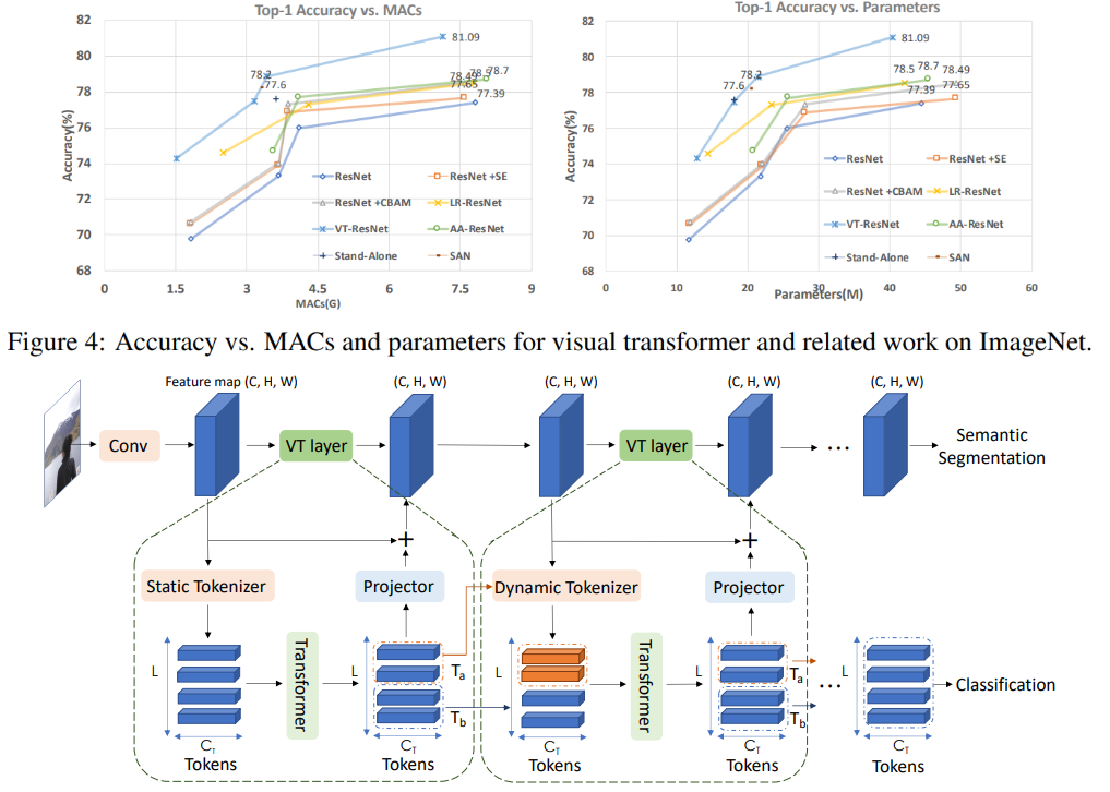
As a result, the authors propose the following: convert images into some kind of visual tokens and submit them to the transformer.

- First, a regular backbone is used to get feature maps
- Next, the feature map is converted into visual tokens
- Tokens are fed to transformers
- Transformer output can be used for classification problems
- And if you combine the output of the transformer with a feature map, you can get predictions for segmentation tasks
Among the works in similar directions, the authors still mention Attention, but notice that usually Attention is applied to pixels, therefore, greatly increases the computational complexity. They also talk about works on improving the efficiency of neural networks, but they believe that in recent years they have provided less and less improvements, so we need to look for other approaches.
Visual transformer
Now let's take a closer look at how the model works.
As mentioned above, the backbone retrieves feature maps, and they are passed to the visual transformer layers.
Each visual transformer consists of three parts: a tokenizer, a transformer, and a projector.
Tokenizer

The tokenizer retrieves visual tokens. In fact, we take a feature map, do a reshape in (H * W, C) and from this we get tokens. The

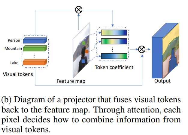
visualization of the coefficients for tokens looks like this:

Position encoding
As usual, transformers need not only tokens, but also information about their position.

First, we do a downsample, then we multiply by the training weights and concatenate with tokens. To adjust the number of channels, you can add 1D convolution.
Transformer
Finally, the transformer itself.

Combining visual tokens and feature map
This makes projector.


Dynamic tokenization
After the first layer of transformers, we can not only extract new visual tokens, but also use those extracted from the previous steps. Trained weights are used to combine them:

Using visual transformers to build computer vision models
Further, the authors describe how the model is applied to computer vision problems. Transformer blocks have three hyperparameters: the number of channels in the feature map C, the number of channels in the visual token Ct, and the number of visual tokens L.
If the number of channels turns out to be unsuitable when switching between the blocks of the model, then 1D and 2D convolutions are used to obtain the required number of channels.
To speed up calculations and reduce the size of the model, use group convolutions.
The authors attach ** pseudocode ** blocks in the article. The full-fledged code is promised to be posted in the future.
Image classification
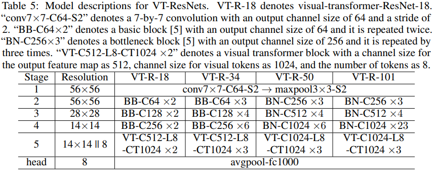
We take ResNet and create visual-transformer-ResNets (VT-ResNet) based on it.
We leave stage 1-4, but instead of the last we put visual transformers.
Backbone exit - 14 x 14 feature map, number of channels 512 or 1024 depending on VT-ResNet depth. 8 visual tokens for 1024 channels are created from the feature map. The output of the transformer goes to the head for classification.

Semantic segmentation
For this task, the panoptic feature pyramid networks (FPN) is taken as a base model.

In FPN, convolutions work on high resolution images, so the model is heavy. The authors replace these operations with visual transformer. Again, 8 tokens and 1024 channels.
Experiments
ImageNet classification
Train 400 epochs with RMSProp. They start with a learning rate of 0.01, increase to 0.16 during 5 warm-up epochs, and then multiply each epoch by 0.9875. Batch normalization and batch size 2048 are used. Label smoothing, AutoAugment, stochastic depth survival probability 0.9, dropout 0.2, EMA 0.99985.
This is how many experiments I had to run to find all this ...
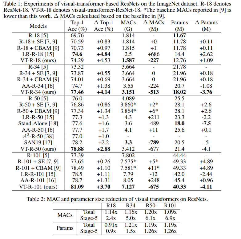
On this graph you can see that the approach gives a higher quality with a reduced number of calculations and the size of the model.


Article titles for compared models:
ResNet + CBAM - Convolutional block attention module
ResNet + SE - Squeeze-and-excitation networks
LR-ResNet - Local relation networks for image recognition
StandAlone - Stand-alone self-attention in vision models
AA-ResNet - Attention augmented convolutional networks
SAN - Exploring self-attention for image recognition
Ablation study
To speed up the experiments, we took VT-ResNet- {18, 34} and trained 90 epochs.

Using transformers instead of convolutions gives the biggest gain. Dynamic tokenization instead of static tokenization also gives a big boost. Position encoding gives only slight improvement.
Segmentation results

As you can see, the metric has grown only slightly, but the model consumes 6.5 times less MAC.
Potential future of the approach
Experiments have shown that the proposed approach allows you to create more efficient models (in terms of computational costs), which at the same time achieve better quality. The proposed architecture successfully works for various tasks of computer vision, and it is hoped that its application will help improve systems using comuter vision - AR / VR, autonomous cars, and others.
The review was prepared by Andrey Lukyanenko, leading developer of MTS.