This is the beginning of a story about how mathematics first invaded geology, how then an IT specialist came and programmed everything, thereby creating a new profession of "digital geologist". This is a story about how stochastic modeling differs from kriging. It is also an attempt to show how you yourself can write your first geological software and, possibly, somehow transform the industry of geological and petroleum engineering.
Let's calculate how much oil is there
, , , , . , , . , (, ). , , , .
— , , , , , , , .
, — . , — . — . , ( , , ) . . , , ( , , ).
. , , , , . — , , . — , , , . , , .
. ; , , , .
, , . , , , , . , .
, , , . , , . , . . , , , - , .
, — , .
, , .. , , . , , , . — — «support». , , , , . .
, , (Krige, D.G. 1951. A statistical approach to some basic mine valuation problems on the Witwatersrand. Journal of the Chemical, Metallurgical and Mining Society of South Africa, December 1951. pp. 119–139.). , -, , , , . , , 5×5 , , , 1 , 50 ×50 ×1 — , , ( — upscaling).
. , — . .
. ,
.
— , . , . , , , .
:
— . (. . 1). , . , . , . , , 1, , .
Python .
import numpy as np
import matplotlib.pyplot as pl

# num of data
N = 5

np.random.seed(0)

# source data
z = np.random.rand(N)
u = np.random.rand(N)

x = np.linspace(0, 1, 100)
y = np.zeros_like(x)

# norm weights
w = np.zeros_like(x)

# power
m = 2

# interpolation
for i in range(N):
    y += z[i] * 1 / np.abs(u[i] - x) ** m
    w += 1 / np.abs(u[i] - x) ** m

# normalization
y /= w

# add source data
x = np.concatenate((x, u))
y = np.concatenate((y, z))
order = x.argsort()
x = x[order]
y = y[order]

# draw graph
pl.figure()

pl.scatter(u, z)
pl.plot(x, y)

pl.show()

pl.close()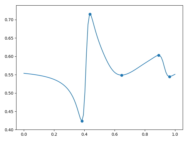
1.
. , , - . , , . -, , , , ? , . , 1 . , , . , , (. . 2). .

2.
, , , , . , , . , . — , , : , , , . , .
(2) :
, , . , , - - . .
, :
- , — . (4) — «», . . , (1):
. , — , — , — «» . , , (6),
(6) ( ). (4) , , dual kriging. (6) (3), , . , (7) , , , , ( ).
(. . 3). , , .
, — Python:
import numpy as np
import matplotlib.pyplot as pl

# num of data
N = 5

np.random.seed(0)

# source data
z = np.random.rand(N) - 0.5
u = np.random.rand(N)

x = np.linspace(0, 1, 100)
y = np.zeros_like(x)

# covariance function
def c(h):
    return np.exp(-np.abs(h ** 2 * 20.))

# covariance matrix
C = np.zeros((N, N))

for i in range(N):
    C[i, :] = c(u - u[i])

# dual kriging weights
lamda = np.linalg.solve(C, z)

# interpolation
for i in range(N):
    y += lamda[i] * c(u[i] - x)

# add source data
x = np.concatenate((x, u))
y = np.concatenate((y, z))
order = x.argsort()
x = x[order]
y = y[order]

# draw graph
pl.figure()

pl.scatter(u, z)
pl.plot(x, y)

pl.show()

pl.close()
3.
, , . (5) (6) , .
, , . , , , .
. , (), , , , . , «», . , (6), , «», . , «» . : . , , , — . , , .
. , . . , , .
.
from theory import probability
from numpy import linalg
, , .
, . () : u , ( ). , .
. . , ( , ).
, - — . - , . : — ( ), , , , . — , .
( , ) . — . , u , .
, , : . -, — «» (4), : . , , .., , , .
, , , , . , , . , , . .
, ( ). :
, , , , . . , , , ( ) , , . . .
, ( , , — , ). , (. . 4).
import numpy as np
import matplotlib.pyplot as pl

np.random.seed(0)

# source data
N = 100
x = np.linspace(0, 1, 100)

# covariance function
def c(h):
    return np.exp(-np.abs(h ** 2 * 250))

# covariance matrix
C = np.zeros((N, N))

for i in range(N):
    C[i, :] = c(x - x[i])

# eigen decomposition
w, v = np.linalg.eig(C)

A = v @ np.diag(w ** 0.5)

# you can check, that C == A @ A.T

# independent normal values
zeta = np.random.randn(N)

# dependent multinormal values
Z = A @ zeta

# draw graph
pl.figure()

pl.plot(x, Z)

pl.show()

pl.close()
4.
, , ( , ). , 5.
import numpy as np
import matplotlib.pyplot as pl

np.random.seed(3)

# source data
M = 5

# coordinates of source data
u = np.random.rand(M)

# source data
z = np.random.randn(M)

# Modeling mesh
N = 100
x = np.linspace(0, 1, N)

# covariance function
def c(h):
return np.exp(−np.abs(h ∗∗ 2 ∗ 250))

# covariance matrix mesh−mesh
Cyy = np.zeros ((N, N))
for i in range (N):
    Cyy[ i , : ] = c(x − x[i])

# covariance matrix mesh−data
Cyz = np.zeros ((N, M))

# covariance matrix data−data
Czz = np.zeros ((M, M))
for j in range (M):
    Cyz [:, j] = c(x − u[j])
    Czz [:, j] = c(u − u[j])

# posterior covariance
Cpost = Cyy − Cyz @ np.linalg.inv(Czz) @ Cyz.T

# lets find the posterior mean, i.e. Kriging interpolation
lamda = np.linalg.solve (Czz, z)
y = np.zeros_like(x)

# interpolation
for i in range (M):
    y += lamda[i] ∗ c(u[i] − x)

# eigen decomposition
w, v = np.linalg.eig(Cpost)
A = v @ np.diag (w ∗∗ 0.5)

# you can check, that Cpost == A@A.T

# draw graph
pl.figure()
for k in range (5):
    # independent normal values
    zeta = np.random.randn(N)
    # dependent multinormal values
    Z = A @ zeta
    pl.plot(x, Z + y, color=[(5 − k) / 5] ∗ 3)
    pl.plot(x, Z + y, color=[(5 − k) / 5] ∗ 3, label=’Stochastic realizations’)

pl.plot(x, y, ’. ’, color=’blue’, alpha=0.4, label=’Expectation(Kriging)’)
pl.scatter(u, z, color=’red ’, label=’Source data’)
pl.legend()
pl.show()
pl.close()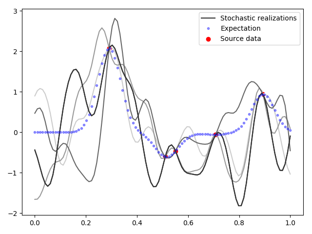
5.
5, . , , , , ( ). , , . — .
, , , (6). , , ( , , ).
, . , . . , , , — . , . — . , - 22 — . -5 , — - . , , , !
?
. (2D 3D), ( 1D ), , , numpy .
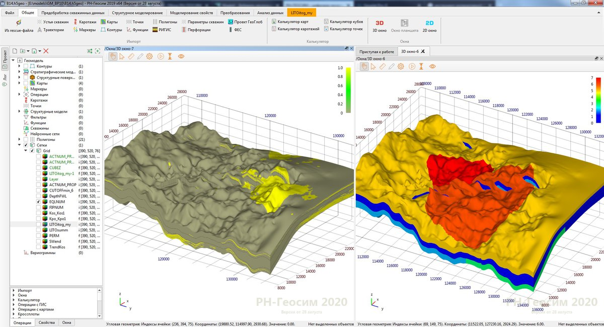
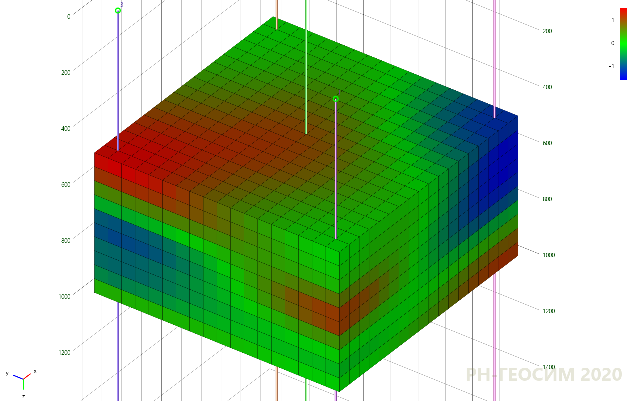
, , 6 «» -.
6. «» -
« ». , . (« ») (. 7) (. 8).
7. «» -
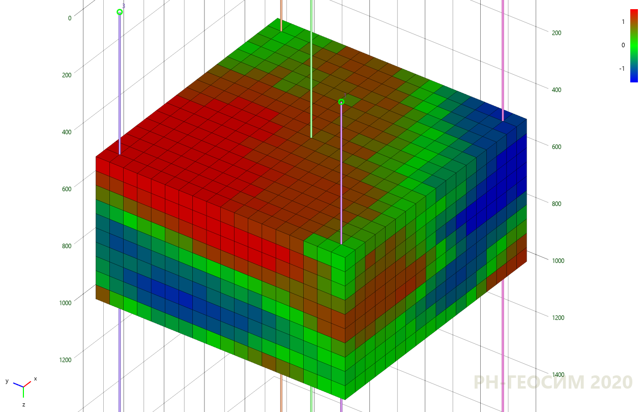
8. «» -
7 8 «» , , , «» .
«»
, . , «X» «Y», . 9.
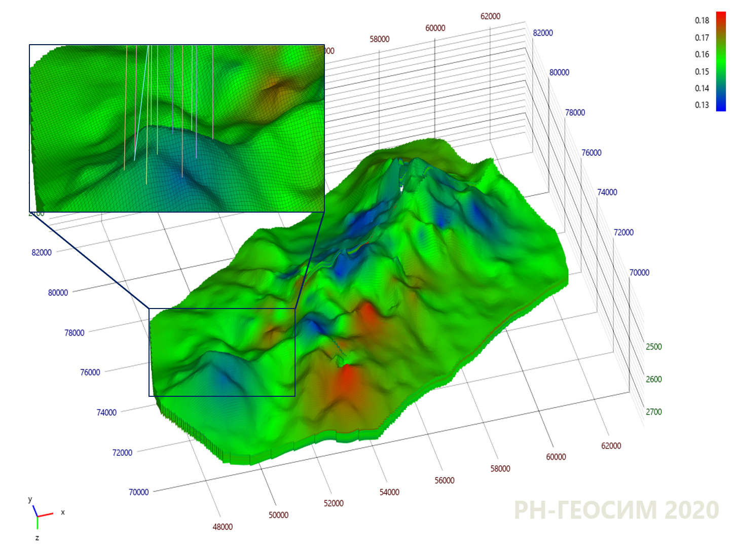
9. "X"
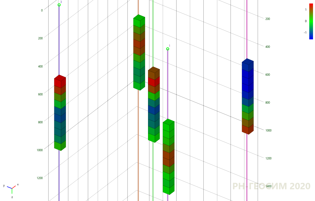
, . , , — ( ). (. . 10).

10. "X"
10 , , - .
, . . , . , .
, , , () , . . ( ), . . , ? , , , :
- ;
- ;
- , .
, - , , , , , , .