
Hello everyone, today we will deal with the JPEG compression algorithm. Many people don't know that JPEG is not so much a format as an algorithm. Most of the JPEG images you see are in JFIF (JPEG File Interchange Format), inside which the JPEG compression algorithm is applied. By the end of the article, you will have a much better understanding of how this algorithm compresses data and how to write unpacking code in Python. We will not consider all the nuances of the JPEG format (for example, progressive scanning), but will only talk about the basic capabilities of the format while we are writing our own decoder.
Introduction
Why write another article on JPEG when hundreds of articles have already been written about it? Usually, in such articles, the authors only talk about what the format is. You don't write unpacking and decoding code. And if you write something, it will be in C / C ++, and this code will not be available to a wide range of people. I want to break this tradition and show you with Python 3 how a basic JPEG decoder works. It will be based on this code developed by MIT, but I'll change it a lot for the sake of readability and clarity. You can find the modified code for this article in my repository .
Different parts of JPEG
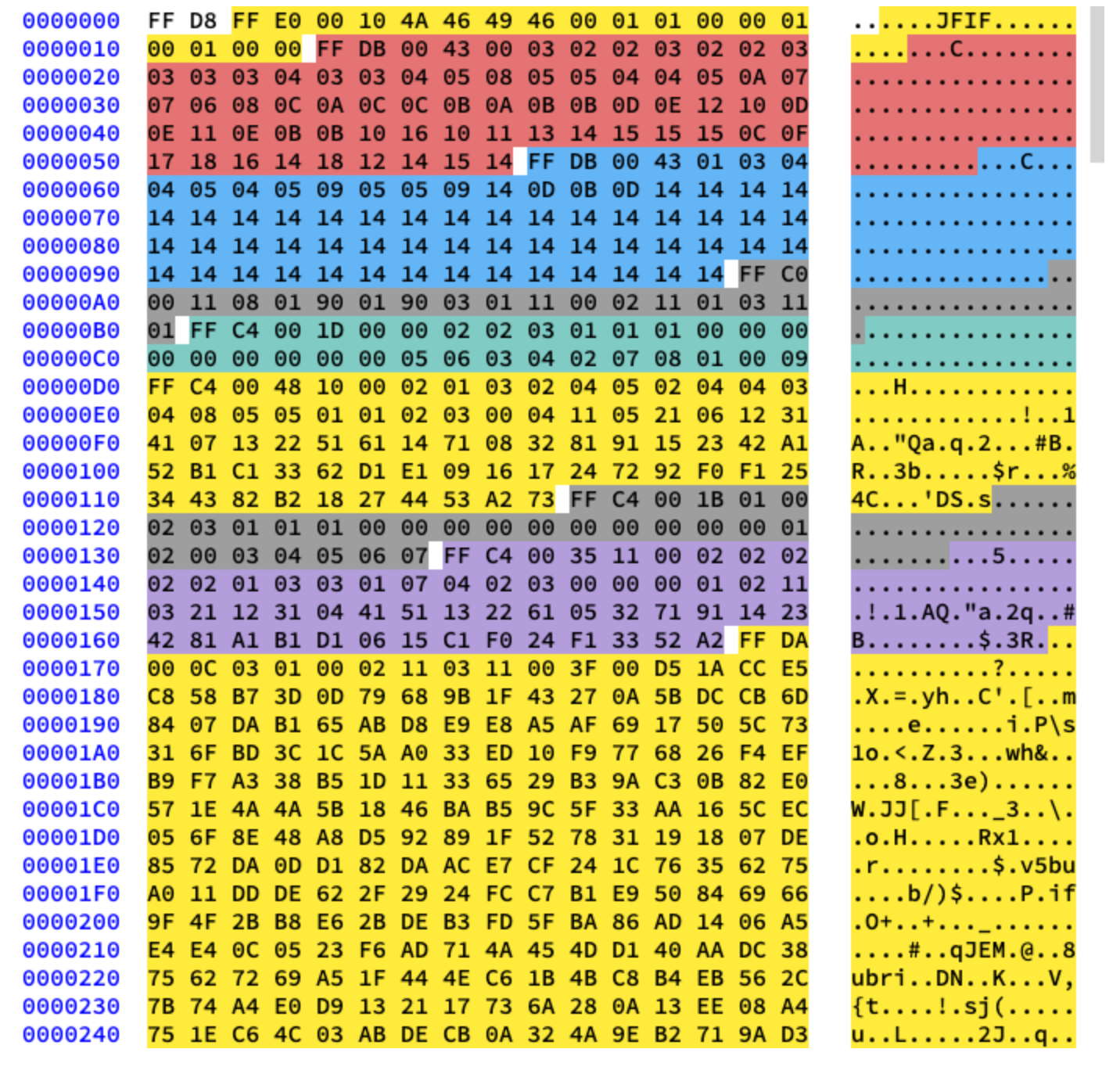
Let's start with a picture made by Ange Albertini . It lists all the parts of a simple JPEG file. We will analyze each segment, and as you read the article, you will return to this illustration more than once.
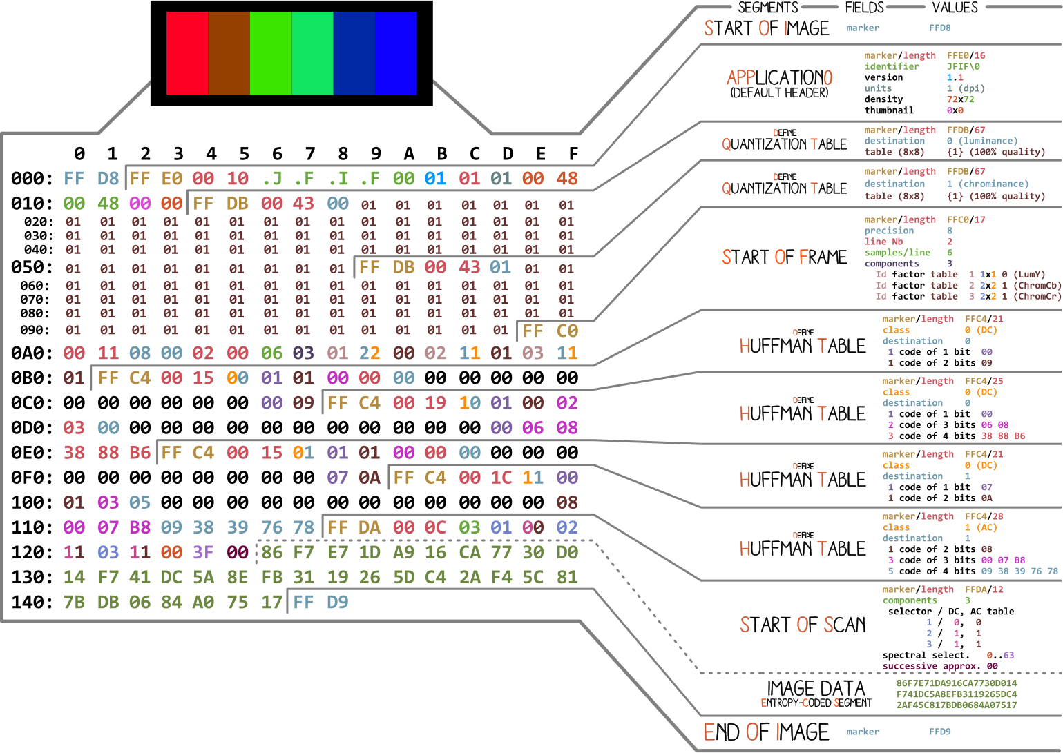
Almost every binary file contains several markers (or headers). You can think of them as some kind of bookmarks. They are essential for working with the file and are used by programs such as file (on Mac and Linux) so that we can find out the details of the file. Markers indicate exactly where certain information is stored in the file. Most often, markers are placed according to the length value (
length) of a particular segment.
Start and end of file
The very first marker important for us is
FF D8. It defines the beginning of the image. If we do not find it, then we can assume that the marker is in some other file. The marker is no less important FF D9. It says that we have reached the end of the image file. After each marker, with the exception of the range FFD0- FFD9and FF01, immediately comes the value of the segment length of this marker. And the markers of the beginning and end of the file are always two bytes long.
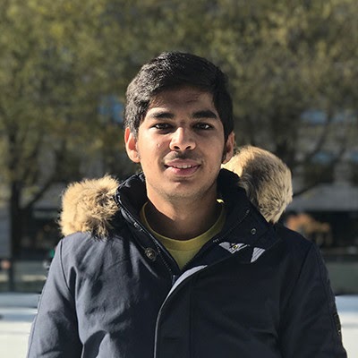
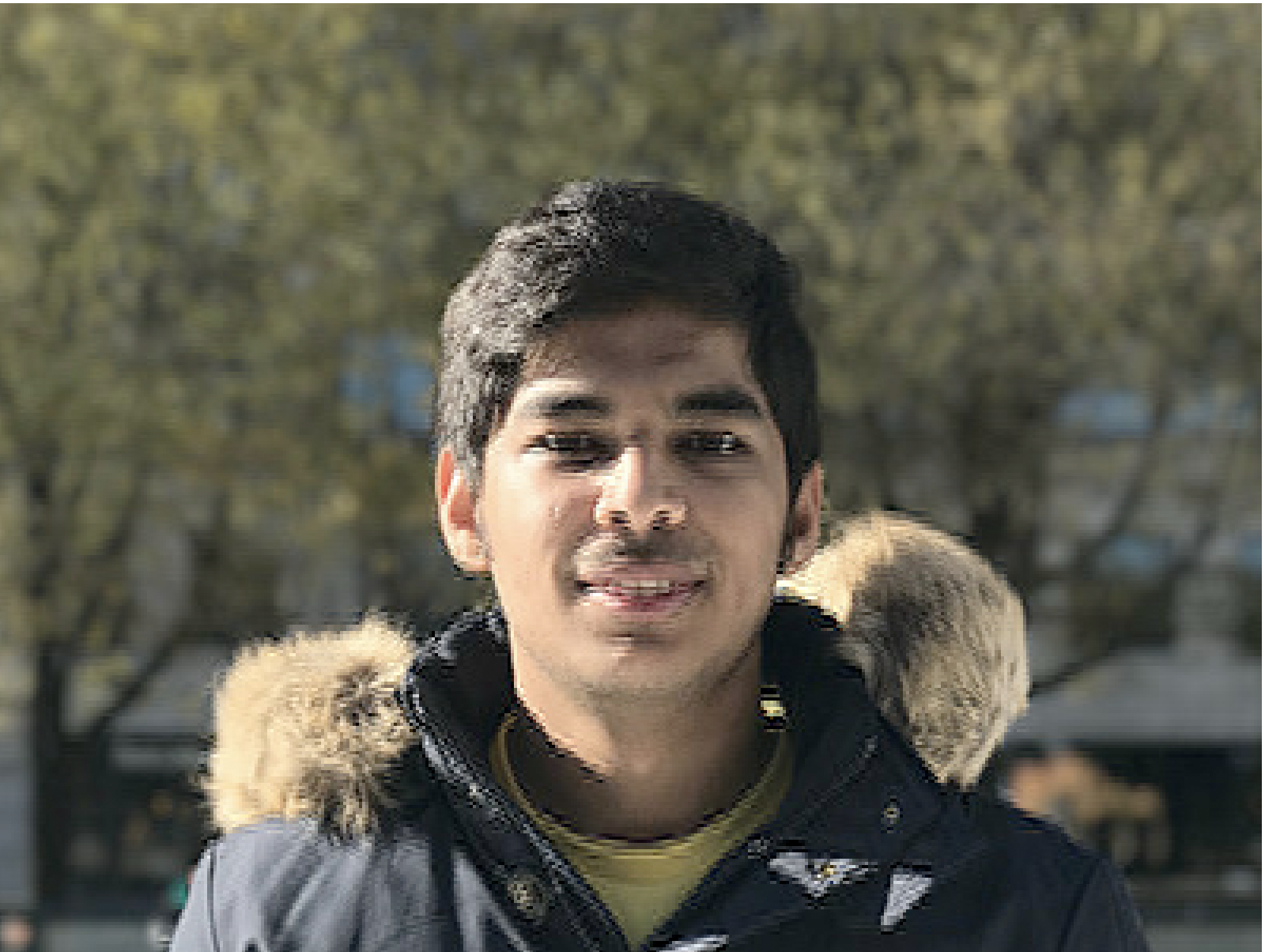
We will be working with this image:
Let's write some code to find the start and end markers.
from struct import unpack

marker_mapping = {
    0xffd8: "Start of Image",
    0xffe0: "Application Default Header",
    0xffdb: "Quantization Table",
    0xffc0: "Start of Frame",
    0xffc4: "Define Huffman Table",
    0xffda: "Start of Scan",
    0xffd9: "End of Image"
}

class JPEG:
    def __init__(self, image_file):
        with open(image_file, 'rb') as f:
            self.img_data = f.read()

    def decode(self):
        data = self.img_data
        while(True):
            marker, = unpack(">H", data[0:2])
            print(marker_mapping.get(marker))
            if marker == 0xffd8:
                data = data[2:]
            elif marker == 0xffd9:
                return
            elif marker == 0xffda:
                data = data[-2:]
            else:
                lenchunk, = unpack(">H", data[2:4])
                data = data[2+lenchunk:]
            if len(data)==0:
                break

if __name__ == "__main__":
    img = JPEG('profile.jpg')
    img.decode()

# OUTPUT:
# Start of Image
# Application Default Header
# Quantization Table
# Quantization Table
# Start of Frame
# Huffman Table
# Huffman Table
# Huffman Table
# Huffman Table
# Start of Scan
# End of Image
To unpack the bytes of the image, we used struct .
>Htells structit to read the data type unsigned shortand work with it in order from high to low (big-endian). JPEG data is stored in the highest to lowest format. Only EXIF data can be in little-endian format (although this is usually not the case). And the size shortis 2, so we transfer unpacktwo bytes from img_data. How did we know what it is short? We know that the markers are in JPEG are denoted by four hexadecimal characters: ffd8. One such character is equivalent to four bits (half a byte), so four characters will be equivalent to two bytes, just like short.
After the Start of Scan section, the scanned image data immediately follows, which does not have a specific length. They continue until the end of file marker, so for now we manually “search” for it when we find the Start of Scan marker.
Now let's deal with the rest of the image data. To do this, we first study the theory, and then move on to programming.
JPEG encoding
First, let's talk about the basic concepts and coding techniques used in JPEG. And coding will be done in reverse order. In my experience, decoding will be difficult to figure out without it.
The illustration below is not yet clear to you, but I will give you hints as you learn the encoding and decoding process. Here's the steps for JPEG encoding ( source ):
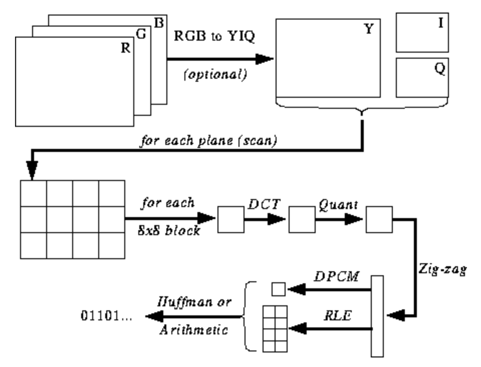
JPEG color space
According to the JPEG specification ( ISO / IEC 10918-6: 2013 (E) Section 6.1):
- Images encoded with only one component are treated as grayscale data, where 0 is black and 255 is white.
- Images encoded with three components are considered RGB data encoded in YCbCr space. If the image contains the APP14 marker segment described in Section 6.5.3, then the color coding is considered RGB or YCbCr according to the information in the APP14 marker segment. The relationship between RGB and YCbCr is defined in accordance with ITU-T T.871 | ISO / IEC 10918-5.
- , , CMYK-, (0,0,0,0) . APP14, 6.5.3, CMYK YCCK APP14. CMYK YCCK 7.
Most implementations of the JPEG algorithm use luminance and chrominance (YUV encoding) instead of RGB. This is very useful because the human eye is very poor at distinguishing high-frequency changes in brightness in small areas, so you can reduce the frequency and the person will not notice the difference. What does it do? Highly compressed image with almost imperceptible quality degradation.
As in RGB, each pixel is encoded with three bytes of colors (red, green and blue), so in YUV, three bytes are used, but their meaning is different. The Y component defines the luminance of the color (luminance, or luma). U and V define the color (chroma): U is responsible for the blue portion, and V for the red portion.
This format was developed at a time when television was not yet so common, and engineers wanted to use the same image encoding format for both color and black-and-white television broadcasting. Read more about this here .
Discrete cosine transform and quantization
JPEG converts the image into 8x8 blocks of pixels (called MCUs, Minimum Coding Unit), changes the range of pixel values so that the center is 0, then applies a discrete cosine transform to each block and compresses the result using quantization. Let's see what all this means.
Discrete cosine transform (DCT) is a method of transforming discrete data into combinations of cosine waves. Converting a picture into a set of cosines looks like a futile exercise at first glance, but you will understand the reason when you learn about the next steps. DCT takes an 8x8 pixel block and tells us how to reproduce that block using a matrix of 8x8 cosine functions. More details here .
The matrix looks like this:
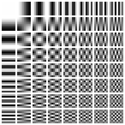
We apply DCT separately to each pixel component. As a result, we get an 8x8 matrix of coefficients, which shows the contribution of each (of all 64) cosine functions in the input 8x8 matrix. In the matrix of DCT coefficients, the largest values are usually in the upper left corner, and the smallest ones are in the lower right. The upper left is the lowest frequency cosine function and the lower right is the highest.
This means that in most images there is a huge amount of low frequency information and a small proportion of high frequency information. If the lower right components of each DCT matrix are assigned a value of 0, then the resulting image will look the same for us, because a person does not distinguish high-frequency changes poorly. This is what we will do in the next step.
I found a great video on this topic. Look if you don't understand the meaning of PrEP:
We all know that JPEG is a lossy compression algorithm. But so far we have not lost anything. We only have blocks of 8x8 YUV components converted to blocks of 8x8 cosine functions without loss of information. The data loss stage is quantization.
Quantization is the process when we take two values from a certain range and turn them into a discrete value. In our case, this is just a sly name for reducing to 0 the highest frequency coefficients in the resulting DCT matrix. When saving an image using JPEG, most graphics editors ask you what level of compression you want to set. This is where the loss of high-frequency information occurs. You will no longer be able to recreate the original image from the resulting JPEG image.
Different quantization matrices are used depending on the compression ratio (fun fact: most developers have patents for creating a quantization table). We divide the DCT matrix of coefficients element by element by the quantization matrix, round the results to integers and get the quantized matrix.
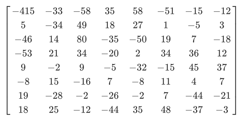
Let's look at an example. Let's say there is such a DCT matrix:
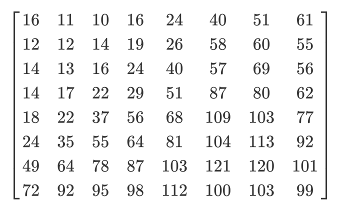
And here is the usual quantization matrix:
The quantized matrix will look like this:
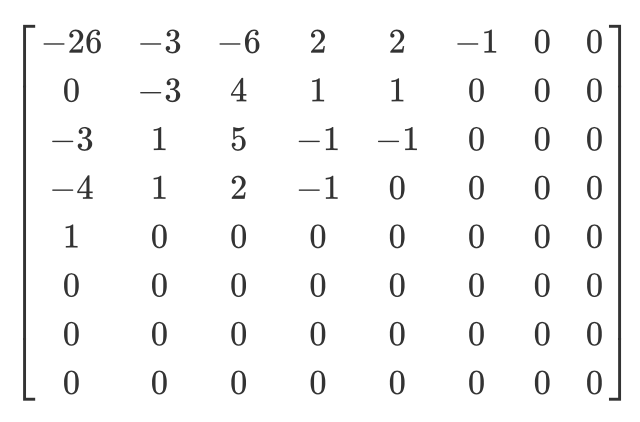
Although the human cannot see the high frequency information, if you remove too much data from the 8x8 pixel blocks, the image will look too rough. In such a quantized matrix, the very first value is called the DC value, and all the others are called AC values. If we took the DC values of all quantized matrices and generated a new image, then we would get a preview with a resolution 8 times smaller than the original image.
I also want to note that since we used quantization, we need to make sure that the colors fall within the range [0.255]. If they fly out of it, then you will have to manually bring them to this range.
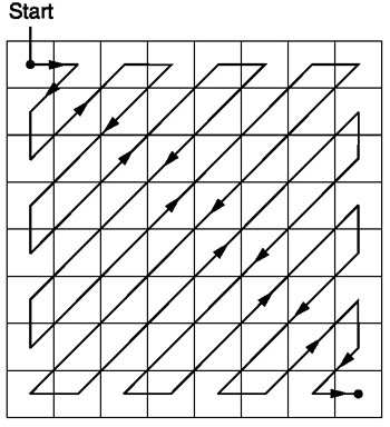
Zigzag
After quantization, the JPEG algorithm uses a zigzag scan to convert the matrix to one-dimensional form:
Source .
Let us have such a quantized matrix:
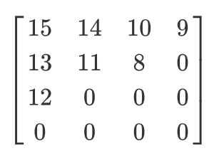
Then the result of the zigzag scan will be as follows:
[15 14 13 12 11 10 9 8 0 ... 0]
This coding is preferred because after quantization, most of the low-frequency (most important) information will be located at the beginning of the matrix, and the zigzag scan stores this data at the beginning of the one-dimensional matrix. This is useful for the next step, compression.
Run-length coding and delta coding
Run-length encoding is used to compress repetitive data. After the zigzag scan, we see that there are mostly zeros at the end of the array. Length encoding allows us to take advantage of this wasted space and use fewer bytes to represent all those zeros. Let's say we have the following data:
10 10 10 10 10 10 10
After encoding the series lengths, we get this:
7 10
We've compressed 7 bytes into 2 bytes.
Delta encoding is used to represent a byte relative to the byte before it. It will be easier to explain with an example. Let us have the following data:
10 11 12 13 10 9
Using delta coding, they can be represented as follows:
10 1 2 3 0 -1
In JPEG, each DC value of the DCT matrix is delta-encoded relative to the previous DC value. This means that by changing the very first DCT coefficient of the image, you will destroy the whole picture. But if you change the first value of the last DCT matrix, then it will only affect a very small fragment of the image.
This approach is useful because the first DC value of the image usually varies the most, and we use delta coding to bring the remaining DC values closer to 0, which improves compression with Huffman coding.
Huffman coding
It is a lossless compression method. One day Huffman wondered, "What is the smallest number of bits I can use to store free text?" As a result, an encoding format was created. Let's say we have text:
a b c d e
Typically, each character takes up one byte of space:
a: 01100001
b: 01100010
c: 01100011
d: 01100100
e: 01100101
This is the principle of binary ASCII encoding. What if we change the mapping?
# Mapping

000: 01100001
001: 01100010
010: 01100011
100: 01100100
011: 01100101
We now need much fewer bits to store the same text:
a: 000
b: 001
c: 010
d: 100
e: 011
That's all well and good, but what if we need to save even more space? For example, like this:
# Mapping
0:  01100001
1:  01100010
00: 01100011
01: 01100100
10: 01100101

a: 0
b: 1
c: 00
d: 01
e: 10
Huffman coding allows such variable length matching. The input data is taken, the most common characters are matched with a smaller combination of bits, and less frequent characters - with larger combinations. And then the resulting mappings are collected into a binary tree. In JPEG, we store DCT information using Huffman coding. Remember I mentioned that delta coding DC values makes Huffman coding easier? I hope you now understand why. After delta encoding, we need to match fewer “characters” and the tree size is reduced.
Tom Scott has a great video explaining how the Huffman algorithm works. Take a look before reading on.
A JPEG contains up to four Huffman tables, which are stored in the "Define Huffman Table" section (starts with
0xffc4). DCT coefficients are stored in two different Huffman tables: in one DC-values from zigzag tables, in the other - AC-values from zigzag tables. This means that when coding, we need to combine the DC and AC values from the two matrices. DCT information for luma and chromaticity channels is stored separately, so we have two sets of DC and two sets of AC information, a total of 4 Huffman tables.
If the image is in grayscale, then we only have two Huffman tables (one for DC and one for AC), because we don't need color. As you might have figured out, two different images can have very different Huffman tables, so it's important to store them inside each JPEG.
We now know the main content of JPEG images. Let's move on to decoding.
JPEG decoding
Decoding can be divided into stages:
- Extraction of Huffman tables and decoding of bits.
- Extracting DCT coefficients using run-length and delta coding rollback.
- Using DCT coefficients to combine cosine waves and reconstruct pixel values for each 8x8 block.
- Convert YCbCr to RGB for each pixel.
- Displays the resulting RGB image.
The JPEG standard supports four compression formats:
- Base
- Extended serial
- Progressive
- No loss
We will work with basic compression. It contains a series of 8x8 blocks following each other. In other formats, the data template is slightly different. To make it clear, I've colored in different segments of the hexadecimal content of our image:
Extracting Huffman Tables
We already know that JPEG contains four Huffman tables. This is the last encoding, so we'll start decoding with it. Each section with the table contains information:
| Field | The size | Description |
|---|---|---|
| Marker ID | 2 bytes | 0xff and 0xc4 identify DHT |
| Length | 2 bytes | Table length |
| Huffman table information | 1 byte | bits 0 ... 3: number of tables (0 ... 3, otherwise error) bit 4: type of table, 0 = DC table, 1 = AC tables bits 5 ... 7: not used, must be 0 |
| Characters | 16 bytes | The number of characters with codes of length 1 ... 16, sum (n) of these bytes is the total number of codes that must be <= 256 |
| Symbols | n bytes | The table contains characters in order of increasing code length (n = total number of codes). |
Let's say we have a Huffman table like this ( source ):
| Symbol | Huffman code | Code length |
|---|---|---|
| a | 00 | 2 |
| b | 010 | 3 |
| c | 011 | 3 |
| d | 100 | 3 |
| e | 101 | 3 |
| f | 110 | 3 |
| g | 1110 | 4 |
| h | 11110 | five |
| i | 111110 | 6 |
| j | 1111110 | 7 |
| k | 11111110 | 8 |
| l | 111111110 | nine |
It will be stored in a JFIF file like this (in binary format. I'm using ASCII for clarity only):
0 1 5 1 1 1 1 1 1 0 0 0 0 0 0 0 a b c d e f g h i j k l
0 means that we have no Huffman code of length 1. A 1 means that we have one Huffman code of length 2, and so on. In the DHT section, immediately after the class and ID, the data is always 16 bytes long. Let's write the code to extract lengths and elements from DHT.
class JPEG:
    # ...

    def decodeHuffman(self, data):
        offset = 0
        header, = unpack("B",data[offset:offset+1])
        offset += 1

        # Extract the 16 bytes containing length data
        lengths = unpack("BBBBBBBBBBBBBBBB", data[offset:offset+16])
        offset += 16

        # Extract the elements after the initial 16 bytes
        elements = []
        for i in lengths:
            elements += (unpack("B"*i, data[offset:offset+i]))
            offset += i

        print("Header: ",header)
        print("lengths: ", lengths)
        print("Elements: ", len(elements))
        data = data[offset:]


    def decode(self):
        data = self.img_data
        while(True):
            # ---
            else:
                len_chunk, = unpack(">H", data[2:4])
                len_chunk += 2
                chunk = data[4:len_chunk]

                if marker == 0xffc4:
                    self.decodeHuffman(chunk)
                data = data[len_chunk:]
            if len(data)==0:
break
After executing the code, we get this:
Start of Image
Application Default Header
Quantization Table
Quantization Table
Start of Frame
Huffman Table
Header:  0
lengths:  (0, 2, 2, 3, 1, 1, 1, 0, 0, 0, 0, 0, 0, 0, 0, 0)
Elements:  10
Huffman Table
Header:  16
lengths:  (0, 2, 1, 3, 2, 4, 5, 2, 4, 4, 3, 4, 8, 5, 5, 1)
Elements:  53
Huffman Table
Header:  1
lengths:  (0, 2, 3, 1, 1, 1, 0, 0, 0, 0, 0, 0, 0, 0, 0, 0)
Elements:  8
Huffman Table
Header:  17
lengths:  (0, 2, 2, 2, 2, 2, 1, 3, 3, 1, 7, 4, 2, 3, 0, 0)
Elements:  34
Start of Scan
End of Image
Excellent! We have lengths and elements. Now you need to create your own Huffman table class in order to reconstruct the binary tree from the obtained lengths and elements. I'll just copy the code from here :
class HuffmanTable:
    def __init__(self):
        self.root=[]
        self.elements = []

    def BitsFromLengths(self, root, element, pos):
        if isinstance(root,list):
            if pos==0:
                if len(root)<2:
                    root.append(element)
                    return True
                return False
            for i in [0,1]:
                if len(root) == i:
                    root.append([])
                if self.BitsFromLengths(root[i], element, pos-1) == True:
                    return True
        return False

    def GetHuffmanBits(self,  lengths, elements):
        self.elements = elements
        ii = 0
        for i in range(len(lengths)):
            for j in range(lengths[i]):
                self.BitsFromLengths(self.root, elements[ii], i)
                ii+=1

    def Find(self,st):
        r = self.root
        while isinstance(r, list):
            r=r[st.GetBit()]
        return  r

    def GetCode(self, st):
        while(True):
            res = self.Find(st)
            if res == 0:
                return 0
            elif ( res != -1):
                return res

class JPEG:
    # -----

    def decodeHuffman(self, data):
        # ----
        hf = HuffmanTable()
        hf.GetHuffmanBits(lengths, elements)
        data = data[offset:]
GetHuffmanBitstakes the lengths and elements, iterates over the elements, and puts them in a list root. It is a binary tree and contains nested lists. You can read on the Internet how the Huffman tree works and how to create such a data structure in Python. For our first DHT (from the picture at the beginning of the article) we have the following data, lengths and elements:
Hex Data: 00 02 02 03 01 01 01 00 00 00 00 00 00 00 00 00
Lengths:  (0, 2, 2, 3, 1, 1, 1, 0, 0, 0, 0, 0, 0, 0, 0, 0)
Elements: [5, 6, 3, 4, 2, 7, 8, 1, 0, 9]
After the call, the
GetHuffmanBitslist rootwill contain the following data:
[[5, 6], [[3, 4], [[2, 7], [8, [1, [0, [9]]]]]]]
HuffmanTablealso contains a method GetCodethat walks through the tree and uses a Huffman table to return the decoded bits. The method receives a bitstream as input - just a binary representation of the data. For example, the bitstream for abcwill be 011000010110001001100011. First, we convert each character to its ASCII code, which we convert to binary. Let's create a class to help convert a string to bits and then count the bits one by one:
class Stream:
    def __init__(self, data):
        self.data= data
        self.pos = 0

    def GetBit(self):
        b = self.data[self.pos >> 3]
        s = 7-(self.pos & 0x7)
        self.pos+=1
        return (b >> s) & 1

    def GetBitN(self, l):
        val = 0
        for i in range(l):
            val = val*2 + self.GetBit()
        return val
When initializing, we give the class binary data and then read it using
GetBitand GetBitN.
Decoding the quantization table
The Define Quantization Table section contains the following data:
| Field | The size | Description |
|---|---|---|
| Marker ID | 2 bytes | 0xff and 0xdb identify the DQT section |
| Length | 2 bytes | Quantization table length |
| Quantization information | 1 byte | bits 0 ... 3: number of quantization tables (0 ... 3, otherwise error) bits 4 ... 7: precision of the quantization table, 0 = 8 bits, otherwise 16 bits |
| Bytes | n bytes | Quantization table values, n = 64 * (precision + 1) |
According to the JPEG standard, a default JPEG image has two quantization tables: for luma and chroma. They start with a marker
0xffdb. The result of our code already contains two such markers. Let's add the ability to decode quantization tables:
def GetArray(type,l, length):
    s = ""
    for i in range(length):
        s =s+type
    return list(unpack(s,l[:length]))

class JPEG:
    # ------
    def __init__(self, image_file):
        self.huffman_tables = {}
        self.quant = {}
        with open(image_file, 'rb') as f:
            self.img_data = f.read()

    def DefineQuantizationTables(self, data):
        hdr, = unpack("B",data[0:1])
        self.quant[hdr] =  GetArray("B", data[1:1+64],64)
        data = data[65:]

    def decodeHuffman(self, data):
        # ------
        for i in lengths:
            elements += (GetArray("B", data[off:off+i], i))
            offset += i
            # ------

    def decode(self):
        # ------
        while(True):
            # ----
            else:
                # -----
                if marker == 0xffc4:
                    self.decodeHuffman(chunk)
                elif marker == 0xffdb:
                    self.DefineQuantizationTables(chunk)
                data = data[len_chunk:]
            if len(data)==0:
                break
We first defined a method
GetArray. It is just a convenient technique for decoding a variable number of bytes from binary data. We also replaced some of the code in the method decodeHuffmanto take advantage of the new function. Then the method was defined DefineQuantizationTables: it reads the title of the section with quantization tables, and then applies the quantization data to the dictionary using the value of the header as the key. this value can be 0 for luminance and 1 for chromaticity. Each section with quantization tables in JFIF contains 64 bytes of data (for an 8x8 quantization matrix).
If we output the quantization matrices for our picture, we get this:
3    2    2    3    2    2    3    3
3    3    4    3    3    4    5    8
5    5    4    4    5    10   7    7
6    8    12   10   12   12   11   10
11   11   13   14   18   16   13   14
17   14   11   11   16   22   16   17
19   20   21   21   21   12   15   23
24   22   20   24   18   20   21   20

3     2    2    3    2    2    3    3
3     2    2    3    2    2    3    3
3     3    4    3    3    4    5    8
5     5    4    4    5    10   7    7
6     8    12   10   12   12   11   10
11    11   13   14   18   16   13   14
17    14   11   11   16   22   16   17
19    20   21   21   21   12   15   23
24    22   20   24   18   20   21   20
Decoding the start of frame
The Start of Frame section contains the following information ( source ):
| Field | The size | Description |
|---|---|---|
| Marker ID | 2 bytes | 0xff 0xc0 SOF |
| 2 | 8 + *3 | |
| 1 | , 8 (12 16 ). | |
| 2 | > 0 | |
| 2 | > 0 | |
| 1 | 1 = , 3 = YcbCr YIQ | |
| 3 | 3 . (1 ) (1 = Y, 2 = Cb, 3 = Cr, 4 = I, 5 = Q), (1 ) ( 0...3 , 4...7 ), (1 ). |
Here we are not interested in everything. We will extract the width and height of the image, as well as the number of quantization tables for each component. The width and height will be used to start decoding the actual scans of the image from the Start of Scan section. Since we will be working mostly with a YCbCr image, we can assume that there will be three components, and their types will be 1, 2 and 3, respectively. Let's write the code to decode this data:
class JPEG:
    def __init__(self, image_file):
        self.huffman_tables = {}
        self.quant = {}
        self.quantMapping = []
        with open(image_file, 'rb') as f:
            self.img_data = f.read()
    # ----
    def BaselineDCT(self, data):
        hdr, self.height, self.width, components = unpack(">BHHB",data[0:6])
        print("size %ix%i" % (self.width,  self.height))

        for i in range(components):
            id, samp, QtbId = unpack("BBB",data[6+i*3:9+i*3])
            self.quantMapping.append(QtbId)

    def decode(self):
        # ----
        while(True):
                # -----
                elif marker == 0xffdb:
                    self.DefineQuantizationTables(chunk)
                elif marker == 0xffc0:
                    self.BaselineDCT(chunk)
                data = data[len_chunk:]
            if len(data)==0:
                break
We added a list attribute to the JPEG class
quantMappingand defined a method BaselineDCTthat decodes the required data from the SOF section and puts the number of quantization tables for each component into the list quantMapping. We'll take advantage of this when we start reading the Start of Scan section. This is how it looks for our picture quantMapping:
Quant mapping: [0, 1, 1]
Decoding Start of Scan
This is the "meat" of a JPEG image, it contains the data of the image itself. We have reached the most important stage. Everything that we decoded before can be considered a card that helps us decode the image itself. This section contains the picture itself (encoded). We read the section and decrypt using the already decoded data.
All markers started with
0xff. This value can also be part of the scanned image, but if it is present in this section, it will always be followed by and 0x00. The JPEG encoder inserts it automatically, this is called byte stuffing. Therefore, the decoder must remove these 0x00. Let's start with the SOS decode method containing such a function and get rid of the existing ones 0x00. In our picture in the section with a scan there is no0xffbut it's still a useful addition.
def RemoveFF00(data):
    datapro = []
    i = 0
    while(True):
        b,bnext = unpack("BB",data[i:i+2])
        if (b == 0xff):
            if (bnext != 0):
                break
            datapro.append(data[i])
            i+=2
        else:
            datapro.append(data[i])
            i+=1
    return datapro,i

class JPEG:
    # ----
    def StartOfScan(self, data, hdrlen):
        data,lenchunk = RemoveFF00(data[hdrlen:])
        return lenchunk+hdrlen

    def decode(self):
        data = self.img_data
        while(True):
            marker, = unpack(">H", data[0:2])
            print(marker_mapping.get(marker))
            if marker == 0xffd8:
                data = data[2:]
            elif marker == 0xffd9:
                return
            else:
                len_chunk, = unpack(">H", data[2:4])
                len_chunk += 2
                chunk = data[4:len_chunk]
                if marker == 0xffc4:
                    self.decodeHuffman(chunk)
                elif marker == 0xffdb:
                    self.DefineQuantizationTables(chunk)
                elif marker == 0xffc0:
                    self.BaselineDCT(chunk)
                elif marker == 0xffda:
                    len_chunk = self.StartOfScan(data, len_chunk)
                data = data[len_chunk:]
            if len(data)==0:
                break
Previously, we manually searched for the end of the file when we found a marker
0xffda, but now that we have a tool that allows us to systematically view the entire file, we will move the marker search condition inside the operator else. The function RemoveFF00just breaks when it finds something else instead of 0x00after 0xff. The loop breaks when the function finds 0xffd9, so we can search for the end of the file without fear of surprises. If you run this code, you will not see anything new in the terminal.
Remember, JPEG splits the image into 8x8 matrices. Now we need to convert the scanned image data to a bitstream and process it in 8x8 chunks. Let's add the code to our class:
class JPEG:
    # -----
    def StartOfScan(self, data, hdrlen):
        data,lenchunk = RemoveFF00(data[hdrlen:])
        st = Stream(data)
        oldlumdccoeff, oldCbdccoeff, oldCrdccoeff = 0, 0, 0
        for y in range(self.height//8):
            for x in range(self.width//8):
                matL, oldlumdccoeff = self.BuildMatrix(st,0, self.quant[self.quantMapping[0]], oldlumdccoeff)
                matCr, oldCrdccoeff = self.BuildMatrix(st,1, self.quant[self.quantMapping[1]], oldCrdccoeff)
                matCb, oldCbdccoeff = self.BuildMatrix(st,1, self.quant[self.quantMapping[2]], oldCbdccoeff)
                DrawMatrix(x, y, matL.base, matCb.base, matCr.base )

        return lenchunk +hdrlen
Let's start by converting the data to a bitstream. Do you remember that delta coding is applied to the DC element of the quantization matrix (its first element) relative to the previous DC element? Therefore, we initialize
oldlumdccoeff, oldCbdccoeffand oldCrdccoeffwith zero values, they will help us keep track of the value of the previous DC-elements, and 0 will be set by default when we find the first DC-element.
The loop
formay seem strange. self.height//8tells us how many times we can divide the height by 8 8, and it's the same with the width and self.width//8.
BuildMatrixwill take a quantization table and add parameters, create an inverse discrete cosine transform matrix and give us the Y, Cr and Cb matrices. And the function DrawMatrixconverts them to RGB.
First, let's create a class
IDCT, and then start filling in the method BuildMatrix.
import math

class IDCT:
    """
    An inverse Discrete Cosine Transformation Class
    """

    def __init__(self):
        self.base = [0] * 64
        self.zigzag = [
            [0, 1, 5, 6, 14, 15, 27, 28],
            [2, 4, 7, 13, 16, 26, 29, 42],
            [3, 8, 12, 17, 25, 30, 41, 43],
            [9, 11, 18, 24, 31, 40, 44, 53],
            [10, 19, 23, 32, 39, 45, 52, 54],
            [20, 22, 33, 38, 46, 51, 55, 60],
            [21, 34, 37, 47, 50, 56, 59, 61],
            [35, 36, 48, 49, 57, 58, 62, 63],
        ]
        self.idct_precision = 8
        self.idct_table = [
            [
                (self.NormCoeff(u) * math.cos(((2.0 * x + 1.0) * u * math.pi) / 16.0))
                for x in range(self.idct_precision)
            ]
            for u in range(self.idct_precision)
        ]

    def NormCoeff(self, n):
        if n == 0:
            return 1.0 / math.sqrt(2.0)
        else:
            return 1.0

    def rearrange_using_zigzag(self):
        for x in range(8):
            for y in range(8):
                self.zigzag[x][y] = self.base[self.zigzag[x][y]]
        return self.zigzag

    def perform_IDCT(self):
        out = [list(range(8)) for i in range(8)]

        for x in range(8):
            for y in range(8):
                local_sum = 0
                for u in range(self.idct_precision):
                    for v in range(self.idct_precision):
                        local_sum += (
                            self.zigzag[v][u]
                            * self.idct_table[u][x]
                            * self.idct_table[v][y]
                        )
                out[y][x] = local_sum // 4
        self.base = out
Let's analyze the class
IDCT. When we extract the MCU, it will be stored in an attribute base. Then we transform the MCU matrix by rolling back the zigzag scan using the method rearrange_using_zigzag. Finally, we will roll back the discrete cosine transform by calling the method perform_IDCT.
As you remember, the DC table is fixed. We will not consider how DCT works, this is more related to mathematics than programming. We can store this table as a global variable and query for pairs of values
x,y. I decided to put the table and its computation in a class IDCTto make the text readable. Each element of the transformed MCU matrix is multiplied by a value idc_variableand we get the Y, Cr, and Cb values.
This will become clearer when we add the method
BuildMatrix.
If you modify the zigzag table to look like this:
[[ 0,  1,  5,  6, 14, 15, 27, 28],
[ 2,  4,  7, 13, 16, 26, 29, 42],
[ 3,  8, 12, 17, 25, 30, 41, 43],
[20, 22, 33, 38, 46, 51, 55, 60],
[21, 34, 37, 47, 50, 56, 59, 61],
[35, 36, 48, 49, 57, 58, 62, 63],
[ 9, 11, 18, 24, 31, 40, 44, 53],
[10, 19, 23, 32, 39, 45, 52, 54]]
you get this result (note the little artifacts):
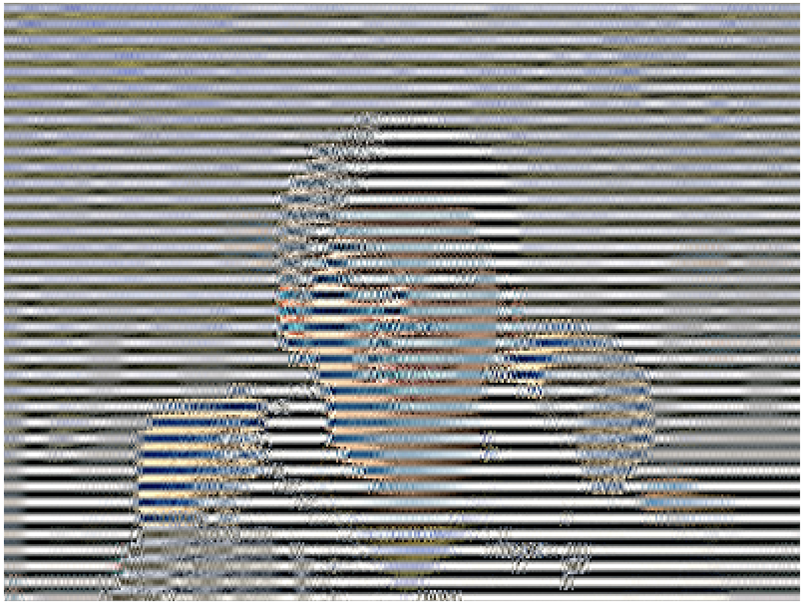
And if you have the courage, you can modify the zigzag table even more:
[[12, 19, 26, 33, 40, 48, 41, 34,],
[27, 20, 13,  6,  7, 14, 21, 28,],
[ 0,  1,  8, 16,  9,  2,  3, 10,],
[17, 24, 32, 25, 18, 11,  4,  5,],
[35, 42, 49, 56, 57, 50, 43, 36,],
[29, 22, 15, 23, 30, 37, 44, 51,],
[58, 59, 52, 45, 38, 31, 39, 46,],
[53, 60, 61, 54, 47, 55, 62, 63]]
Then the result will be like this:
Let's complete our method
BuildMatrix:
def DecodeNumber(code, bits):
    l = 2**(code-1)
    if bits>=l:
        return bits
    else:
        return bits-(2*l-1)


class JPEG:
    # -----
    def BuildMatrix(self, st, idx, quant, olddccoeff):
        i = IDCT()

        code = self.huffman_tables[0 + idx].GetCode(st)
        bits = st.GetBitN(code)
        dccoeff = DecodeNumber(code, bits) + olddccoeff

        i.base[0] = (dccoeff) * quant[0]
        l = 1
        while l < 64:
            code = self.huffman_tables[16 + idx].GetCode(st)
            if code == 0:
                break

            # The first part of the AC quantization table
            # is the number of leading zeros
            if code > 15:
                l += code >> 4
                code = code & 0x0F

            bits = st.GetBitN(code)

            if l < 64:
                coeff = DecodeNumber(code, bits)
                i.base[l] = coeff * quant[l]
                l += 1

        i.rearrange_using_zigzag()
        i.perform_IDCT()

        return i, dccoeff
We start by creating a discrete cosine transform invert class (
IDCT()). Then we read the data into the bitstream and decode it using a Huffman table.
self.huffman_tables[0]and self.huffman_tables[1]refer to DC tables for luma and chroma, respectively, and self.huffman_tables[16]and self.huffman_tables[17]refer to AC tables for luma and chroma, respectively.
After decoding the bitstream, we use a function to
DecodeNumber extract the new delta-coded DC coefficient and add to it olddccoefficientto get the delta-decoded DC coefficient.
We then repeat the same decoding procedure with the AC values in the quantization matrix. Code meaning
0indicates that we have reached the End of Block (EOB) marker and must stop. Moreover, the first part of the AC quantization table tells us how many leading zeros we have. Now let's remember about coding the lengths of the series. Let's reverse this process and skip all those many bits. IDCTThey are explicitly assigned zeros in the class .
After decoding the DC and AC values for the MCU, we convert the MCU and invert the zigzag scan by calling
rearrange_using_zigzag. And then we invert the DCT and applied to the decoded MCU.
The method
BuildMatrixwill return the inverted DCT matrix and the value of the DC coefficient. Remember that this will be a matrix for only one minimum 8x8 encoding unit. Let's do this for all the other MCUs in our file.
Displaying an image on the screen
Now let's make our code in the method
StartOfScancreate a Tkinter Canvas and draw each MCU after decoding.
def Clamp(col):
    col = 255 if col>255 else col
    col = 0 if col<0 else col
    return  int(col)

def ColorConversion(Y, Cr, Cb):
    R = Cr*(2-2*.299) + Y
    B = Cb*(2-2*.114) + Y
    G = (Y - .114*B - .299*R)/.587
    return (Clamp(R+128),Clamp(G+128),Clamp(B+128) )

def DrawMatrix(x, y, matL, matCb, matCr):
    for yy in range(8):
        for xx in range(8):
            c = "#%02x%02x%02x" % ColorConversion(
                matL[yy][xx], matCb[yy][xx], matCr[yy][xx]
            )
            x1, y1 = (x * 8 + xx) * 2, (y * 8 + yy) * 2
            x2, y2 = (x * 8 + (xx + 1)) * 2, (y * 8 + (yy + 1)) * 2
            w.create_rectangle(x1, y1, x2, y2, fill=c, outline=c)

class JPEG:
    # -----
    def StartOfScan(self, data, hdrlen):
        data,lenchunk = RemoveFF00(data[hdrlen:])
        st = Stream(data)
        oldlumdccoeff, oldCbdccoeff, oldCrdccoeff = 0, 0, 0
        for y in range(self.height//8):
            for x in range(self.width//8):
                matL, oldlumdccoeff = self.BuildMatrix(st,0, self.quant[self.quantMapping[0]], oldlumdccoeff)
                matCr, oldCrdccoeff = self.BuildMatrix(st,1, self.quant[self.quantMapping[1]], oldCrdccoeff)
                matCb, oldCbdccoeff = self.BuildMatrix(st,1, self.quant[self.quantMapping[2]], oldCbdccoeff)
                DrawMatrix(x, y, matL.base, matCb.base, matCr.base )

        return lenchunk+hdrlen


if __name__ == "__main__":
    from tkinter import *
    master = Tk()
    w = Canvas(master, width=1600, height=600)
    w.pack()
    img = JPEG('profile.jpg')
    img.decode()
    mainloop()
Let's start with functions
ColorConversionand Clamp. ColorConversiontakes Y, Cr and Cb values, converts them to RGB components by the formula, and then outputs the aggregated RGB values. Why add 128 to them, you might ask? Remember, before the JPEG algorithm, DCT is applied to the MCU and subtracts 128 from the color values. If the colors were originally in the range [0.255], JPEG will put them in the range [-128, + 128]. We need to roll back this effect when decoding, so we add 128 to RGB. As for Clamp, when unpacking, the resulting values may go outside the range [0.255], so we keep them in this range [0.255].
In method
DrawMatrixwe loop through each decoded 8x8 matrix for Y, Cr and Cb, and convert each matrix element to RGB values. After transforming, we draw pixels in Tkinter canvasusing the method create_rectangle. You can find all the code on GitHub . If you run it, my face will appear on the screen.
Conclusion
Who would have thought that to show my face you would have to write an explanation of more than 6,000 words. It's amazing how clever the authors of some of the algorithms were! Hope you enjoyed the article. I learned a lot while writing this decoder. I didn't think there was so much math involved in encoding a simple JPEG image. Next time you can try writing a decoder for PNG (or another format).
Additional materials
If you are interested in the details, read the materials that I used to write the article, as well as some additional work: