A Gantt chart is a collection of horizontal bars on a plane. The horizontal direction corresponds to the value of time, and this value, in the general case, can be continuous. And in the vertical direction, this plane is divided into many horizontal zones of fixed width. For the classic Gantt chart, reflecting the work schedule, each such zone corresponds to a certain type of work (Fig. 1). Chart bars are plotted within these zones. The strip depicted in a specific zone characterizes the type of work corresponding to this zone, and the left and right borders of the strip characterize, respectively, the start and end times of this work. Therefore, the length of the strip characterizes the duration of the given work.

Figure: 1. Gantt chart to illustrate the work schedule.
In the case of the diagram of telephone calls described in this article, the zones in the vertical direction will characterize days (days). In this case, the horizontal time scale of the diagram corresponds to the interval from 0 to 24 hours, one day long. Each bar in such a diagram would correspond to one phone call. The left and right boundaries of the lane are the start and end times of the call, and the zone number (vertically) is the day when the call was made. A diagram of such a configuration allows you to visually illustrate and evaluate how often calls are made, to estimate their average duration, distribution by time of day, etc. Moreover, one more property can be added to this diagram: the color of the bar. You can color the stripes according to different criteria. First, by the type of call (incoming or outgoing).Secondly - by the phone number of the call. In the first case, two colors are enough. In the second - much more, but, as a rule, no more than a dozen colors are enough for the most popular phone numbers that appear in calls most often. This article describes the formation of a chart for a period of five calendar months and taking into account the presence of two mobile operators (two-SIM phone). The colors of the bars on the diagram will be selected on the basis of "SIM1 / SIM2 incoming / outgoing", that is, four different colors are required.This article describes the formation of a chart for a period of five calendar months and taking into account the presence of two mobile operators (two-SIM phone) The colors of the bars on the diagram will be selected on the basis of "SIM1 / SIM2 incoming / outgoing", that is, four different colors are required.This article describes the formation of a chart for a period of five calendar months and taking into account the presence of two mobile operators (two-SIM phone). The colors of the bars on the diagram will be selected on the basis of "SIM1 / SIM2 incoming / outgoing", that is, four different colors are required.
Formation of a diagram, in contrast to construction, provides for the generation of an output file with a given diagram. As for plotting, as a rule, building a chart in Excel would imply the corresponding operation in Excel, one of the standard tools. Even if such an operation is possible (Gantt chart), it is unlikely to be convenient to display and scale on large volumes of input data. In the case of generating an SVG vector file with a similar diagram, Excel is used as a software tool where it is convenient to work with tabular data. Instead of Excel, you could write a third-party separate program and generate an SVG file using it. But Excel in this case I chose not by chance. Firstly, in a way, there is a certain visualization of information processing,and secondly, the specificity of the SVG output format.
This format is a scalable vector graphics format and contains XML-formatted text data inside. It is a kind of markup language that contains a specific set of commands and parameters that are typical for drawing a particular graphic element. Commands, for example, can be as follows: draw a line, polygon, circle, write text. And the parameters are the coordinates of the corners of the polygon, the fill color, the size and font of the text, etc. In fact, knowing the SVG markup language, you can use a regular text editor (Notepad) to manually create one or another picture from the category of the simplest. SVG files can be opened for viewing with any common Internet browser.
Before proceeding with the formation of the SVG diagram, it is necessary not only to download the call details from the sites of mobile operators, but also to pre-process them. As I already noted, two mobile operators will be considered. One of them is Tele2, the other is Megafon. Detailing of Tele2 calls, which can be downloaded from your personal account on the corresponding website, is a PDF document with a large table, which is divided into pages (Fig. 2).

Figure: 2. Type of call detailing "Tele2".
In the case of Megafon, everything is almost the same, except that the details are presented in the XLS (Excel) file (Fig. 3).

Figure: 3. Type of call detailing "Megafon".
Both the one and the other detailing must be processed in different ways, weed out unnecessary and put in order. This text has a certain "regularity", so it is easily subject to automatic processing. I produced it in a separate document using Excel functions (formulas). I don't think it is worth dwelling on this issue in detail. As a result of such processing, we got a neat large table with the minimum required fields: date, time, duration, type of call, phone number, sim card (Fig. 4). A total of 2102 phone call records were obtained. By the way, in Figure 3, which shows an Excel sheet with the original detailing text, you can see the presence of other sheets. I added these sheets just to implement the intermediate stages of processing, as a continuation of the original document.

Figure: 4. Mixed detailing, put in order.
I copied the resulting table into a new document on sheet "A", immediately supplementing it with additional fields: the address of the stripe color, the left border of the stripe (a) (in seconds from the beginning of the day), the right border of the stripe (b) (Fig. 5).

Figure: 5. Additional parameters on the first sheet.
These fields are easily calculated using Excel formulas. The color address indicates one of the four addresses of the cells of the configuration sheet "C", in which it is written in the HEX-RGB format. This sheet contains not only colors, but also all additional parameters of the SVG document: coordinates, offsets, scale, etc. (fig. 6).

Figure: 6. Sheet with parameters.
In addition to the bars, the diagram will display additional data: the allocation of the four most frequent telephone numbers with a separate label on the bar, a histogram of the distribution of the frequency of telephone calls in time, as well as information about the diagram.
Looking ahead, the diagram is 4420 by 1800 pixels. It's actually difficult to talk about pixels in vector graphics, but in the description of the SVG format, there is a discrete coordinate system, the counts of which I call pixels. In general, even based on the abbreviation, this graphics is scalable. As I already wrote, the diagram will reflect calls for 5 months, namely, from May to September inclusive. If you count it, this corresponds to 153 days. There should be exactly the number of zones for the bars on the diagram. I decided in advance on the scale. In the vertical direction, I decided to allot 10 pixels per zone. In this case, the width of the strip in the zone will be 8 pixels, (with a gap of one pixel at the top and bottom). The size of the gap (indentation) in cell B8 of the sheet "C" can adjust the width of the stripes in the zone. The horizontal scale can be chosen, in principle, any,however, there is a practical clarity of the diagram, an acceptable aspect ratio and capacity. In the end, I decided to take 3 pixels for the length of one minute, or in other words, 20 seconds per pixel.
In total, the active area of the chart has the following dimensions. Horizontal: 24 * 60 * 3 = 4320; vertical: 153 * 10 = 1530. On the left of the diagram, opposite each zone should be written its name. The zone names are fully consistent with the dates. For this purpose, I decided to set aside a 100px wide area. Above the diagram, it is desirable (for convenience) to write timestamps, at least hours. And below, under the chart, there will be a histogram about which I wrote above, as well as additional information. For these purposes, I allotted 270 pixels, rounding the height of the entire diagram to 1800. In addition to all that has been said, on the diagram I decided to reflect light horizontal lines between zones (days), a little darker - between weeks, and black - between months. In addition to horizontal lines, there are also vertical lines, placed every hour - for the boundaries of the hours.And one more important detail. On the left border of each displayed color strip, a black mark of its beginning will be displayed in the form of a square opening bracket. This is necessary in order to prevent the merging of two bands, which can correspond to consecutive telephone calls.
The main processing of information occurs on sheet "B" (Fig. 7). There you can see a bunch of "extra" intermediate pillars, the values of the cells of which could be calculated "in the head" or immediately taken into account in the final formula. This concerns the coordinates of the corners of each strip. However, it all seemed to me very cumbersome, which at first could be confusing.

Figure: 7. Sheet with basic calculations.
Column "A" extracts the day (zone) number from the call date. Column "B" - call time in seconds from the beginning of the day. This is the same value as in column "I" of sheet "C". Column "C" - rounded up call duration in minutes. Here it is worth making a reservation, for which such an "inaccuracy" was introduced. It would seem that you need to take the duration of the call with an accuracy of 20 seconds, that is, up to one pixel of the diagram (based on the accepted scale). However, it is obvious that very short stripes 1-2 pixels wide will not display well on the chart. Therefore, the minimum stripe length will correspond to at least three pixels. In general, the length of any strip will be a multiple of three. By rounding the call duration up (with an accuracy of a minute), the diagram will be slightly "crowded" in comparison with the real situation,however, this overflow is very minor. In column "D" using the formula "INDIRECT", the color value is extracted from the parameters (Sheet "C") at the calculated address on sheet "A". Next, the coordinates of the strip corners are calculated. As I already wrote, there are a lot of unnecessary intermediate calculations, but I didn't redo it. Column "U" calculates the presence of highlighting and the color of the band border if the telephone number of the current call matches one of the four given telephone numbers for highlighting (on sheet "C"). I forgot to write above that in the selected call, not only a label is superimposed on the corresponding strip, but also the gray color of the strip border (this color can also be changed on the sheet with parameters). In the normal case, the strip has no edging. Finally,in the next three columns, the final formation of the text in the SVG graphics markup language takes place. In this article, I will not consider the description and syntax of this language. In fact, this is not difficult, I figured it out in a few minutes. In the "V" column, a code is generated that draws a strip with a border.
Example:
<path fill="#FF5050" stroke="#808080" d="M1598,51L1598,59L1601,59L1601,51L1598,51" style="stroke-width: 1px;" stroke-width="1" stroke-dasharray="0"></path>.
Column "W" contains the code for the left edge of the strip.
Example:
<path fill="none" stroke="black" d="M1599,52L1598,52L1598,58L1599,58" style="stroke-width: 1px;" stroke-width="1" stroke-dasharray="0"></path>.
Column "X" contains the code for displaying the label text (number 1, 2, 3 or 4) only for those calls where it is needed. This selectivity is performed using the formula "IF (U2 <>" none "; ...; ...)".
Sample text "3":
<text x="1601" y="58" style="text-anchor: middle; font-family: times; font-weight: bolder; font-size: 8px;" stroke="none" fill="black"><tspan>3</tspan></text>.
Figure 8 shows a screenshot of these three columns at a very small scale, since otherwise it is almost impossible to demonstrate due to the bulk of the text. You can also see how cumbersome it is to write the CONCATENATE formula with all its arguments.
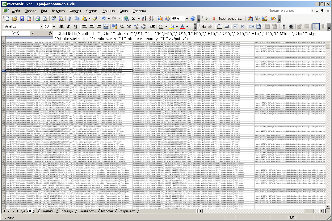
Figure: 8. Columns with the results of basic calculations.
On the "Inscriptions" sheet, inscriptions are formed above the diagram (hour markers) and to the left of the diagram (date) (Fig. 9). The formulas contain font parameters: size, style, font color and border. The main focus of the calculation is automatic filling of cells by dates and hours, calculating the coordinates of the position of the text through a uniform step.

Figure: 9. Sheet forming the inscriptions.
On the "Borders" sheet, all auxiliary lines of the diagram are formed, which serve as the boundaries of zones (dates) and hours. Figure 10 shows a screenshot showing the formation of horizontal lines by zones. The first two columns contain the zone number (starting from zero) and its relative vertical coordinate. The third column generates the SVG code that draws the lines. Here, in the formation of the code, not only the familiar formula "CONNECT" is used, but also two formulas "IF", nested one inside the other. This is necessary to implement a line drawing of three different colors, depending on the situation. As stated above, black lines separate months, gray - weeks, and light gray - days. The last two colors are specified on sheet “C” in cells B17 and C17. In the arguments of the formula "IF" there are formulas "DAY" and "OSTAT". The first formula recognizes a number from a date given as an integer,which is obtained by shifting the values of the zone number (from the first column) by the preselected constant 42491.
In particular, a check is made for the equality of a number from a date with a unit, thereby recognizing the beginning of a new month. The "OSTAT" formula is used to recognize the beginning of a new week (classic algorithm). The second argument of this formula is 7, since there are 7 days in a week. In particular, the remainder of the division is compared with the value 1. This value (from 0 to 6) can be used to adjust the shift of the days of the week on the diagram, and it is selected in such a way that it matches the real calendar. After the formation of horizontal lines, 25 vertical lines are formed in a simpler way (23 lines for every hour and two more boundary lines).
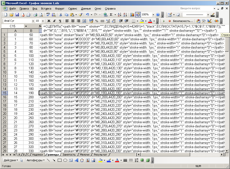
Figure: 10. Sheet that forms the borders.
The sheet "Little things" (Fig. 11) contains the formation of additional information about the properties of the diagram. Columns "B" and "C" contain the offset coordinates for each element.

Figure: 11. Sheet forming additional information.
On the "Occupancy" tab, a histogram of the distribution of calls density over time is formed (Fig. 12). It is a collection of vertical lines of various lengths, which are closely adjacent to each other and located directly below the diagram. The number of such lines corresponds to the number of time elements (20 seconds each), namely 24 * 60 * 3 = 4320.

Figure: 12. Sheet that forms a histogram of call density.
The length of the line (the height of the bar of the histogram) exactly corresponds to the sum of the "occupied" time elements for all 153 days. That is, if a phone call falls on the current time element in the current day, then it is taken into account in the histogram. I calculated such a numeric array using a separate simple C program. With the help of Excel cells, such a calculation cannot be done due to the multidimensionality of operations. It was possible to use VBA by placing the corresponding program code there, but at that time I did not own this tool at all. The program code for calculating the array of histogram values is given below.
#include <stdio.h>
#include <windows.h>

int main(){
	int a,b,n,c,k;
	int q[4320];
	for(n=0;n<4320;n++){
		q[n]=0;
	}
	FILE *f,*f1;
	f=fopen("ab.txt","r");
	f1=fopen("Out.txt","w");
	for(c=0;c<2102;c++){
		fscanf(f,"%i\t%i\n",&a,&b);
		for(k=a;k<b;k++){
			q[k/20]+=1;
		}
	}
	for(n=0;n<4320;n++){
		fprintf(f1,"%i\n",q[n]);
	}
	fclose(f);
	fclose(f1);
	system("PAUSE");
	return 0;
}
The input data of the program is the text file "ab.txt". Two columns from sheet “A” of values of seconds of the beginning and end of each call have been copied into this file (I already wrote about this above, see Fig. 5). The calculated array values are output to the "Out.txt" output file. The calculation algorithm is simple, so there is no need to describe it. The data from the output file is copied to column "D" on the "Employment" worksheet. The first three columns are the legend of the elements of the time intervals and their number. Column "E" - the same value of the histogram, but scaled 5 times, rounded to the nearest integer. This is done for convenient placement of the histogram, clarity and elimination of bulkiness. In addition, each value is offset by one. This is necessary for pseudo drawing of the horizontal axis. Even if the histogram value is zero (which is typical for night time),one pixel of the histogram will still be displayed. Thus, the abscissa axis will be drawn.
Finally, the Result sheet combines all generated SVG codes for each sheet of the document in a specific order (labels and borders first). I made this union using the usual manual column copying (fig. 13). If necessary, you can write in VBA a function to automatically export the SVG file, going through the resulting columns of all sheets. The very first line contains the file header. It contains, first of all, the width and height of the picture. The very last line, added by hand, closes the document, or rather the main svg block. There were about 6800 lines in total.

Figure: 13. Worksheet with the consolidation of results.
Then you need to copy the entire contents of this sheet into a text editor (I used the AkelPad program) and save the document to a file with the svg extension in UTF-8 encoding. After that, if there are no errors, the file is opened in the Internet browser for viewing. The figures below show views of different areas of the resulting image at different scales.

Figure: 14. General view of the resulting diagram in Chrome.
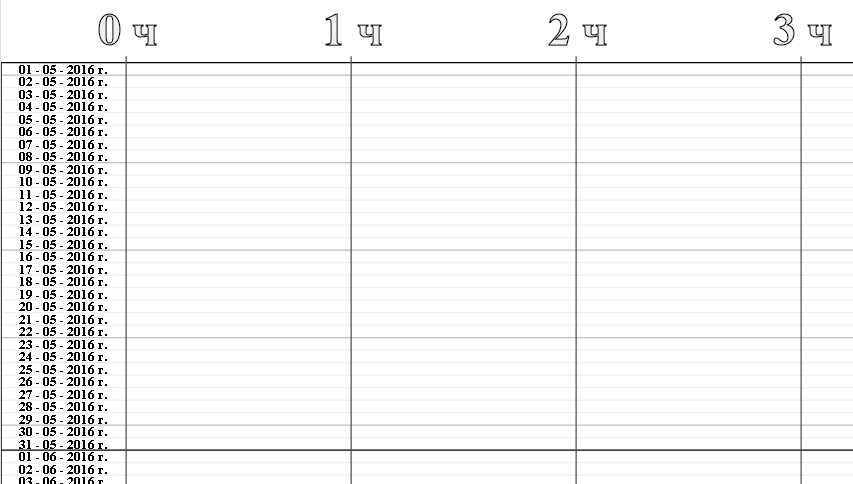
Figure: 15. Upper left corner of the diagram (types of different boundaries and names of zones).

Figure: 16. Chart bars with labels.

Figure: 17. The bars of the chart and the bar graph below them.

Figure: 18. Additional information on the diagram.

Figure: 19. Chart bars and hour markers above them.