This small volume of work was urgently performed for educational and demonstration purposes about a year ago on the basis of an already developed string model. As usual, then after lying idle for a certain time, she recently caught my eye.
There is no point in telling what Scilab is - the reader knows how to use the Internet.

Interesting for the reader already familiar with Scilab, this work can be a rather non-trivial application of this tool. This refers to the "finite element" approach to system modeling and animation display of the results with an oscilloscope. Of course, there are tools specially "sharpened" for mechanics, but, I repeat, the goal was to urgently test Scilab.
For those who were not familiar with this simple and visual tool before, it will be interesting to know this. The whole process of mastering this previously unfamiliar type of software (visual programming), from the moment of installing the free Xcos to the creation of the following text, took me five days. A simpler model of a system with one degree of freedom was finally ready on the second day. And for you, I think, things in the study of this software environment, if desired, will go no worse, so go for it.
The text itself is, perhaps, too laconic, since it was not originally intended for a wide audience. But if the reader has any questions, I will try to remember the details and answer these questions. So.
The mechanical system ("vibrating string in a viscous medium"), considered in detail in this article , represents the following:
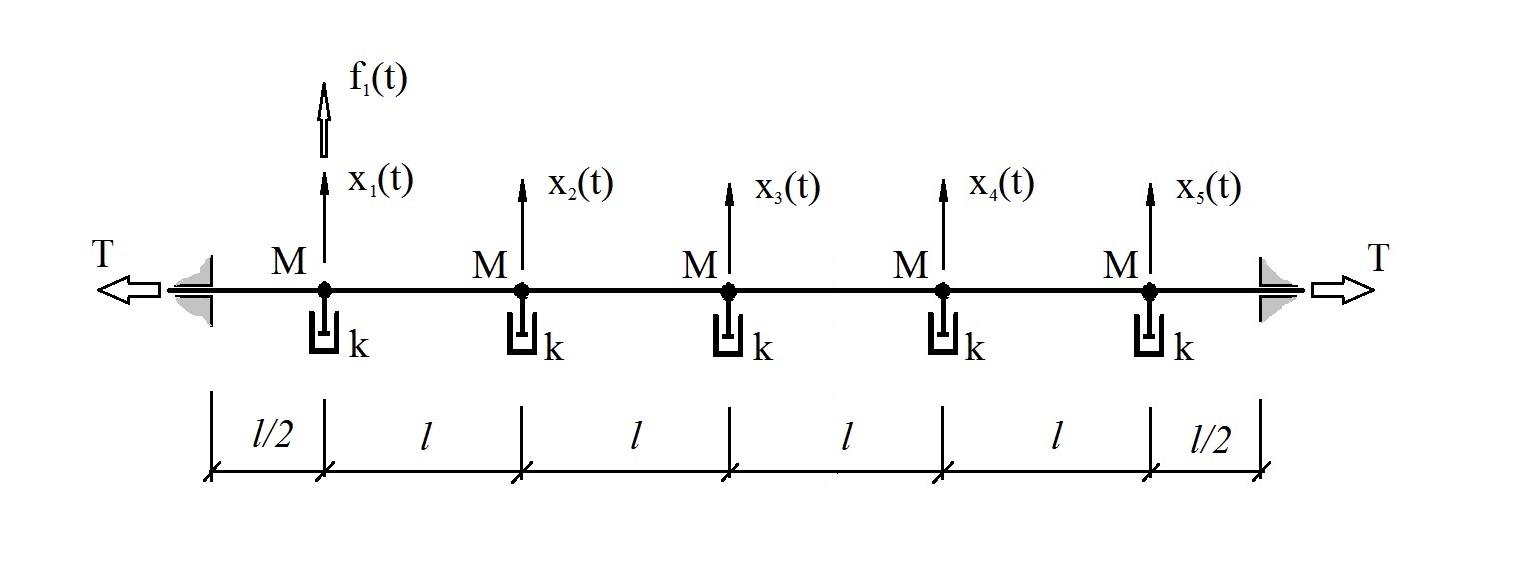
where Δt = 0.01s, l = 1m, M = 1kg, k = 10 kg / s, T = 2000H
To simplify modeling and expanding the possibilities of modifying the model, the model is broken down into such elements that

were modeled as subsystems ("superblocks").
The following "diagram" (model) is built in the visual programming system Xcos
The "diagram" (model) allows you to simulate the behavior of the system under the influence of a single impulse applied to the node (element) No. 1, register and graphically display the external influence in the node No. 1 and the response (displacement) of the system in the nodes No. 1,2,3, and also visually display the behavior of the system in the form of an animated conditional image.
Each of the five "superblocks" (subsystems) included in the "diagram" represents the following

The block receives from the main system data on external influences, lengths and displacements of conjugated elements, clock time, the value of the time sampling interval and the string tension. The block in its settings contains data on its length, mass and damping coefficient, which can be changed for simulation purposes. (The possibility of block concealment declared by the Xcos developer was not realized due to, apparently, software malfunctions.)
The block integrates the corresponding linear ODE by the finite difference method. Zero initial integration conditions are implemented using the Xcos system defaults.
The block transmits data about its movements (in system clock time) and length (constant) to the main system.
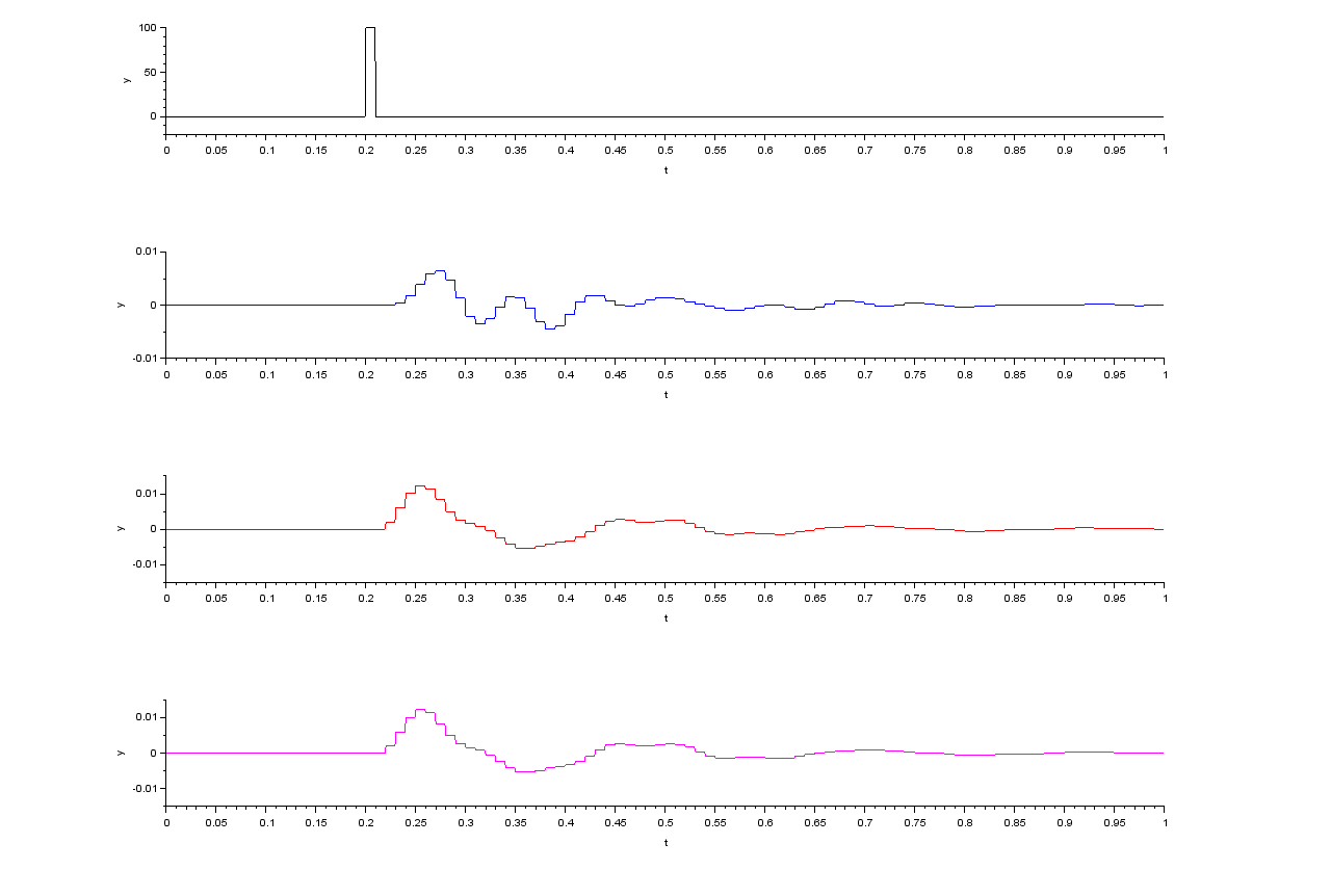
The following results of simulation modeling were obtained.

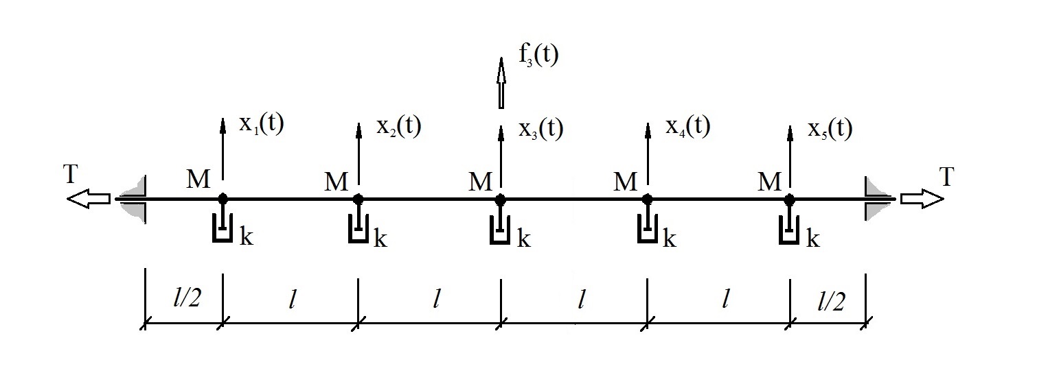
Further, for the purpose of a more complete disclosure of the resonance properties of the system, a simulation was performed similar to the previous one, with an external influence applied to the middle of the string (at node No. 3).

The following results of simulation modeling were obtained:

That's all. Good luck in learning Scilab, everyone.