Self-identification
My name is Alexander, I am developing the direction of data and technology analytics for the purposes of internal audit of the Rosbank group. My team and I use machine learning and neural networks to identify risks as part of internal audit audits. We have a server ~ 300 GB RAM and 4 processors with 10 cores in our arsenal. For algorithmic programming or modeling, we use Python.
Introduction
We were faced with the task of analyzing photographs (portraits) of clients taken by bank employees during the registration of a banking product. Our goal is to identify previously uncovered risks from these photographs. To identify risk, we generate and test a set of hypotheses. In this article, I will describe what hypotheses we came up with and how we tested them. To simplify the perception of the material, I will use Mona Lisa - the standard of the portrait genre.

Check sum
At first, we took an approach without machine learning and computer vision, just comparing the checksums of the files. To generate them, we took the widely used md5 algorithm from the hashlib library.
Python * implementation:
#
with open(file,'rb') as f:
    #
    for chunk in iter(lambda: f.read(4096),b''):
        #
        hash_md5.update(chunk)
When forming the checksum, we immediately check for duplicates using a dictionary.
#
for file in folder_scan(for_scan):
    #
    ch_sum = checksum(file)
    #
    if ch_sum in list_of_uniq.keys():
        #    , ,     dataframe
        df = df.append({'id':list_of_uniq[chs],'same_checksum_with':[file]}, ignore_index = True)
This algorithm is incredibly simple in terms of computational load: on our server 1000 images are processed in no more than 3 seconds.
This algorithm helped us identify duplicate photos among our data, and as a result, find places for potential improvement of the bank's business process.
Key points (computer vision)
Despite the positive result of the checksum method, we understood perfectly well that if at least one pixel in the image is changed, its checksum will be radically different. As a logical development of the first hypothesis, we assumed that the image could be changed in bit structure: undergo resave (that is, re-compression of jpg), resize, crop or rotate.
For demonstration, let's crop the edges along the red outline and rotate the Mona Lisa 90 degrees to the right.

In this case, duplicates must be searched for by the visual content of the image. For this, we decided to use the OpenCV library, a method for constructing key points of an image and finding the distance between key points. In practice, key points can be corners, color gradients, or surface jogs. For our purposes, one of the simplest methods came up - Brute-Force Matching. To measure the distance between the key points of the image, we used the Hamming distance. The picture below shows the result of finding key points on the original and modified images (20 key points of the images closest in distance are drawn).
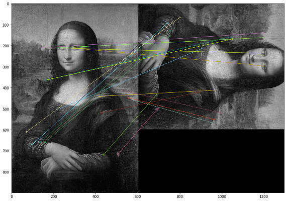
It is important to note that we are analyzing images in a black and white filter, as this optimizes the script runtime and gives a more unambiguous interpretation of key points. If one image is with a sepia filter and the other is in a color original, then when we convert them to a black and white filter, the key points will be identified regardless of the color processing and filters.
Sample code to compare two images *
img1 = cv.imread('mona.jpg',cv.IMREAD_GRAYSCALE)          #
img2 = cv.imread('mona_ch.jpg',cv.IMREAD_GRAYSCALE) #
#  ORB
orb = cv.ORB_create()
#      ORB
kp1, des1 = orb.detectAndCompute(img1,None)
kp2, des2 = orb.detectAndCompute(img2,None)

#  Brute-Force Matching
bf = cv.BFMatcher(cv.NORM_HAMMING, crossCheck=True)
#   .
matches = bf.match(des1,des2)
#    .
matches = sorted(matches, key = lambda x:x.distance)

#     20
img3 = cv.drawMatches(img1,kp1,img2,kp2,matches[:20],None,flags=cv.DrawMatchesFlags_NOT_DRAW_SINGLE_POINTS)

plt.imshow(img3),plt.show()
While testing the results, we realized that in the case of flip image, the order of pixels within the key point changes and such images are not identified as the same. As a compensatory measure, you can mirror each image yourself and analyze double the volume (or even triple), which is much more expensive in terms of computing power.
This algorithm has a high computational complexity, and the operation of calculating the distance between points creates the greatest load. Since we have to compare each image with each, then, as you understand, the calculation of such a Cartesian set requires a large number of computational cycles. In one audit, a similar calculation took over a month.
Another problem with this approach was the poor interpretability of test results. We get the coefficient of the distances between the key points of the images, and the question arises: "What threshold of this coefficient should be chosen sufficient to consider the images duplicated?"
Using computer vision, we were able to find cases that were not covered by the first checksum test. In practice, these turned out to be oversaved jpg files. We did not identify more complex cases of image changes in the analyzed dataset.
Checksum VS key points
Having developed two radically different approaches to finding duplicates and reusing them in several checks, we came to the conclusion that for our data the checksum gives a more tangible result in a shorter time. Therefore, if we have enough time to check, then we make a comparison by key points.
Search for abnormal images
After analyzing the results of the test for key points, we noticed that photographs taken by one employee have approximately the same number of close key points. And this is logical, because if he communicates with clients at his workplace and takes pictures in the same room, then the background on all his photos will be the same. This observation led us to believe that we can find exception photos that are unlike other photos of this employee, which may have been taken outside the office.
Returning to the example with Mona Lisa, it turns out that other people will appear against the same background. But, unfortunately, we did not find such examples, so in this section we will show data metrics without examples. To increase the speed of computation in the framework of testing this hypothesis, we decided to abandon key points and use histograms.
The first step is to translate the image into an object (histogram) that we can measure in order to compare the images by the distance between their histograms. Basically, a histogram is a graph that gives an overview of the image. This is a graph with pixel values on the abscissa axis (X axis) and the corresponding number of pixels in the image along the ordinate axis (Y axis). A histogram is an easy way to interpret and analyze an image. Using the histogram of a picture, you can get an intuitive idea of contrast, brightness, intensity distribution, and so on.
For each image, we create a histogram using the calcHist function from OpenCV.
histo = cv2.calcHist([picture],[0],None,[256],[0,256])
In the examples given for three images, we described them using 256 factors along the horizontal axis (all types of pixels). But we can also rearrange the pixels. Our team didn't do a lot of tests in this part as the result was pretty good when using 256 factors. If necessary, we can change this parameter directly in the calcHist function.
After we have created histograms for each image, we can simply train the DBSCAN model on images for each employee who photographed the client. The technical point here is to select the DBSCAN parameters (epsilon and min_samples) for our task.
After using DBSCAN, we can do image clustering, and then apply the PCA method to visualize the resulting clusters.

As can be seen from the distribution of the analyzed images, we have two pronounced blue clusters. As it turned out, on different days an employee can work in different offices - photographs taken in one of the offices create a separate cluster.
Whereas the green dots are exception photos where the background is different from these clusters.
Upon detailed analysis of the photographs, we found many wrongly negative photos. The most common cases are blown out photographs or photographs in which a large percentage of the area is occupied by the client's face. It turns out that this method of analysis requires mandatory human intervention to validate the results.
Using this approach, you can find interesting anomalies in the photo, but it will take an investment of time to manually analyze the results. For these reasons, we rarely run such tests as part of our audits.
Is there a face in the photo? (Face Detection)
So, we have already tested our dataset from different sides and, continuing to develop the complexity of testing, we move on to the next hypothesis: is there a face of the prospective client in the photo? Our task is to learn how to identify faces in pictures, give functions to the input of a picture and get the number of faces at the output.
This kind of implementation already exists, and we decided to choose MTCNN (Multitasking Cascade Convolutional Neural Network) for our task from the FaceNet module from Google.
FaceNet is a deep machine learning architecture that consists of convolutional layers. FaceNet returns a 128-dimensional vector for each face. In fact, FaceNet is several neural networks and a set of algorithms for preparing and processing intermediate results of these networks. We decided to describe the mechanics of face search by this neural network in more detail, since there are not so many materials about this.
Step 1: preprocessing
The first thing MTCNN does is create multiple sizes of our photo.
MTCNN will try to recognize faces within a fixed size square in each photograph. Using this recognition on the same photo of different sizes will increase our chances of correctly recognizing all the faces in the photo.

A face may not be recognized in a normal image size, but it may be recognized in a different size image in a fixed size square. This step is performed algorithmically without a neural network.
Step 2: P-Net
After creating different copies of our photo, the first neural network, P-Net, comes into play. This network uses a 12x12 kernel (block) that will scan all photos (copies of the same photo, but different sizes), starting from the upper left corner, and move along the picture using a 2 pixel increment.

After scanning all images of different sizes, MTCNN again standardizes each photo and recalculates the block coordinates.
The P-Net gives the coordinates of the blocks and the confidence levels (how accurately this face is) relative to the face it contains for each block. You can leave blocks with a certain level of trust using the threshold parameter.
At the same time, we cannot simply select the blocks with the maximum level of trust, because the picture can contain several faces.
If one block overlaps another and covers almost the same area, then that block is removed. This parameter can be controlled during network initialization.

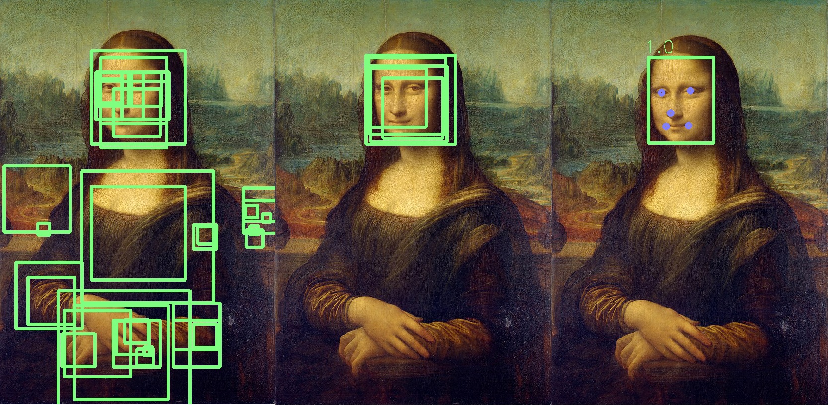
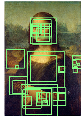
In this example, the yellow block will be removed. Basically, the result of the P-Net is low precision blocks. The example below shows the real results of P-Net:
Step 3: R-Net
R-Net performs a selection of the most suitable blocks formed as a result of the work of P-Net, which in the group is most likely a person. R-Net has a similar architecture to P-Net. At this stage, fully connected layers are formed. The output from R-Net is also similar to the output from P-Net.

Step 4: O-Net
The O-Net network is the last part of the MTCNN network. In addition to the last two networks, it forms five points for each face (eyes, nose, corners of the lips). If these points completely fall into the block, then it is determined as the most likely containing the person. Additional points are marked in blue:

As a result, we get a final block indicating the accuracy of the fact that this is a face. If the face is not found, then we will get zero number of face blocks.
On average, processing of 1000 photos by such a network takes 6 minutes on our server.
We have repeatedly used this neural network in checks, and it helped us to automatically identify anomalies among the photographs of our clients.
About using FaceNet, I would like to add that if, instead of Mona Lisa, you start analyzing Rembrandt's canvases, the results will be something like the image below, and you will have to parse the entire list of identified persons:

Conclusion
These hypotheses and testing approaches demonstrate that with absolutely any data set, you can perform interesting tests and look for anomalies. Many auditors are now trying to develop similar practices, so I wanted to show practical examples of the use of computer vision and machine learning.
I would also like to add that we considered Face Recognition as the next hypothesis for testing, but so far the data and process specifics do not provide a reasonable basis for using this technology in our tests.
In general, this is all that I would like to tell you about our path in testing photos.
I wish you good analytics and labeled data!
* The sample code is taken from open sources.