Part 2
In this article, you will learn:
- About ImageNet Large Scale Visual Recognition Challenge (ILSVRC)
- About what CNN architectures exist:
- LeNet-5
- AlexNet
- VGGNet
- GoogLeNet
- ResNet
- About what problems appeared with new network architectures, how they were solved by subsequent ones:
- vanishing gradient problem
- exploding gradient problem
ILSVRC
The ImageNet Large Scale Visual Recognition Challenge is an annual competition in which Researchers compare their grids for object detection and classification in photographs.
This competition was the impetus for the development of:
- Neural network architectures
- personal methods and practices that are used to this
day.This graph shows how classification algorithms have evolved over time:
On the x-axis - years and algorithms (since 2012 - convolutional neural network).
The y-axis is the percentage of errors in the sample from top-5 error.
Top-5 error is a way of evaluating the model: the model returns a certain probability distribution and if among the top-5 probabilities there is a true value (class label) of the class, then the model's answer is considered correct. Accordingly, (1 - top-1 error) is the familiar accuracy.
CNN architectures
LeNet-5
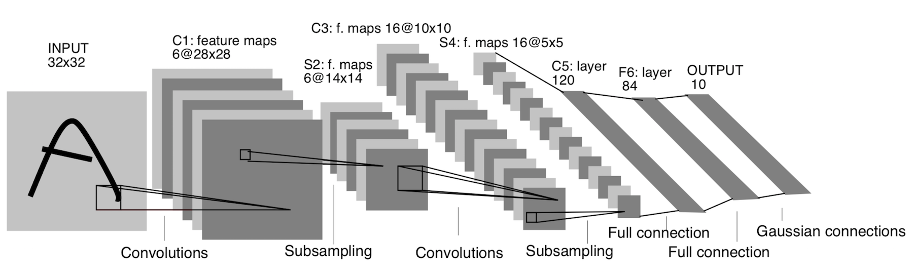
It appeared already in 1998! It was designed to recognize handwritten letters and numbers. Subsampling here refers to the pooling layer.
Architecture:
CONV 5x5, stride = 1
POOL 2x2, stride = 2
CONV 5x5, stride = 1
POOL 5x5, stride = 2
FC (120, 84)
FC (84, 10)
Now this architecture has only historical significance. This architecture is easy to implement by hand in any modern deep learning framework.
AlexNet

The picture is not duplicated. This is how the architecture is depicted, because the AlexNet architecture did not fit on one GPU device at that time, so "half" of the network was running on one GPU, and the other on the other.
It appeared in 2012. A breakthrough in that very ILSVRC began with her - she defeated all stat-of-art models of that time. After that, people realized that neural networks really work :)
Architecture more specifically:

If you look closely at the AlexNet architecture, you can see that for 14 years (since the appearance of LeNet-5), almost no changes have occurred, except for the number of layers.
Important:
- We take our original 227x227x3 image and lower its dimensions (in height and width), but increase the number of channels. This part of the architecture "encodes" the original representation of the object (encoder).
- ReLU. ReLu .
- 60 .
- .
:
- Local Response Norm — , . batch-normalization.
- - , — - FLOPs, .
- FC 4096 , (Fully-connected) 4096 .
- Max Pool 3x3s2 , 3x3, = 2.
- A record like Conv 11x11s4, 96 means that the convolution layer has a 11x11xNc filter, step = 4, the number of such filters is 96. Now the number of such filters is the number of channels for the next layer (the same Nc). We assume that the initial image has three channels (R, G and B).
VGGNet
Architecture:
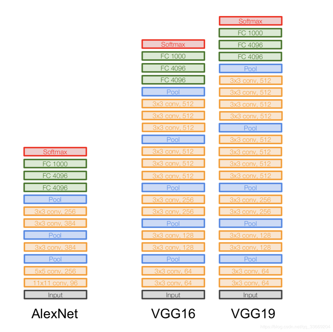
Introduced in 2014.
Two versions - VGG16 and VGG19. The basic idea is to use small ones (3x3) instead of large ones (11x11 and 5x5). The intuition for using large convolutions is simple - we want to get more information from neighboring pixels, but it is much better to use small filters more often .
And that's why:
- . , . .. , , .
- => .
- — , — , — , .
Important:
- When training a neural network for an error backpropagation algorithm, it is important to preserve object representations (for us, the original image) at all stages (convolutions, pools) of forward propagation (forward pass is when we feed the image to the input and move to the output, to the result). This representation of an object can be expensive in terms of memory. Take a look:
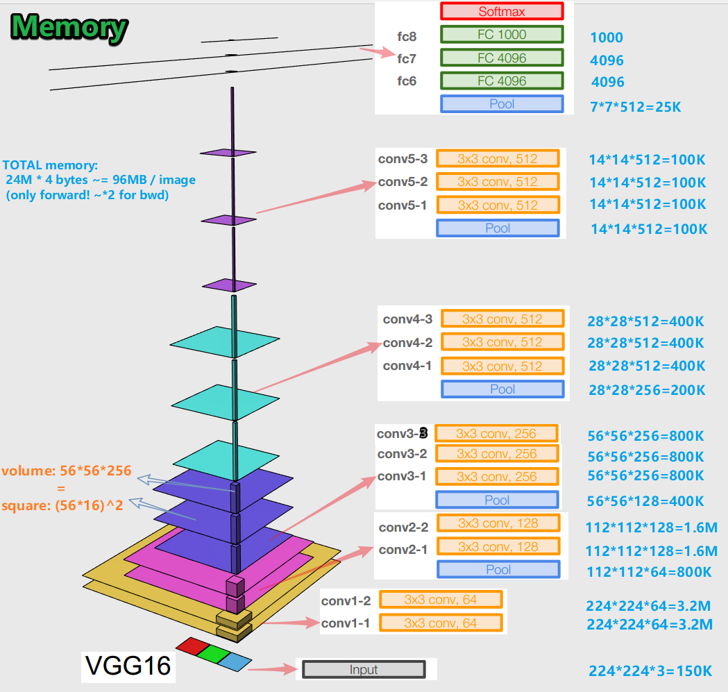
It turns out about 96 MB per image - and that's just for the forward pass. For the backward pass (bwd in the picture) - during the calculation of gradients - about twice as much. An interesting picture emerges: the largest number of trained parameters is located in fully connected layers, and the largest memory is occupied by object representations after convolutional and pooling layers . C - synergy.
- The network has 138 million training parameters in 16 layers variation and 143 million parameters in 19 layers variation.
GoogLeNet
Architecture:
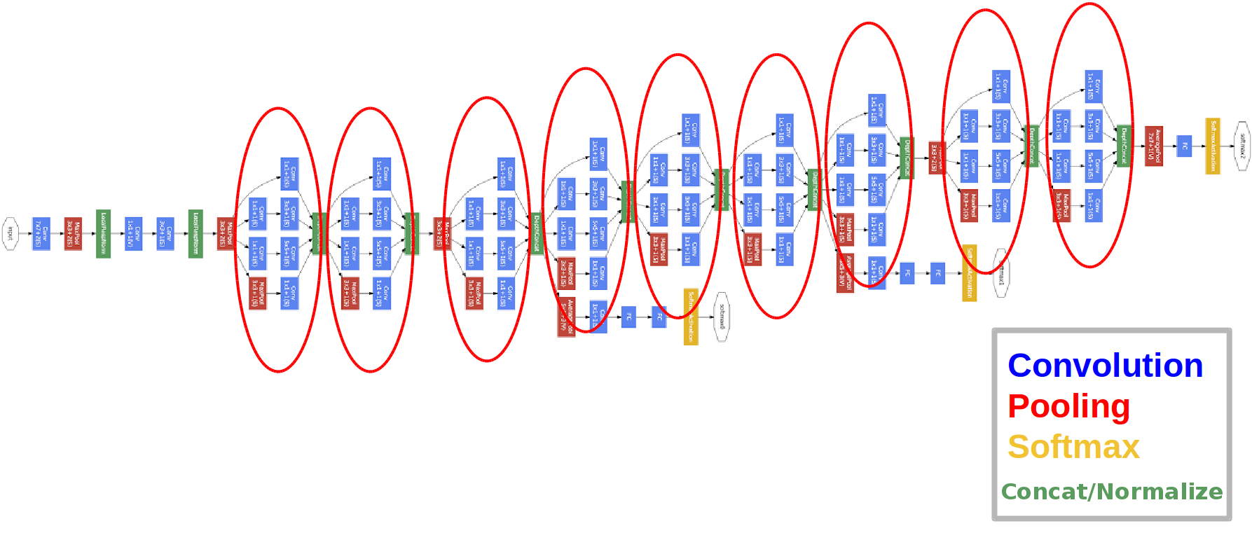
Introduced in 2014.
The red circles are the so-called Inception module.
Let's take a closer look at it:
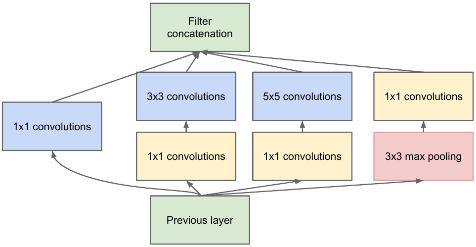
We take a feature map from the previous layer, apply a number of convolutions with different filters to it, then concatenate the resulting one. The intuition is simple: we want to get different representations of our feature map using filters of different sizes. Convolutions 1x1 are used in order not to increase the number of channels so much after each such inception block. Those. when the feature map has a large number of channels, and they want to reduce this number without changing the height and width of the feature map, use the 1x1 convolution.
There are also three classifier blocks in the network, this is how one of them looks like (the one on the right for us):

With this construction, the gradient "better" reaches from the output layers to the input layers during the backpropagation of the error.
Why do we need two extra network outputs? It's all about the so-called vanishing gradient problem :
The bottom line is that when backpropagating an error, the gradient tends to trivially to zero. The deeper the network, the more susceptible it is to this phenomenon. Why it happens? When we backward pass, we go from output to input, calculating the gradients of complex functions. Derivative of a complex function ( chain rule) Is essentially multiplication. And so, multiplying some values along the way from the output to the input, we meet numbers that are close to zero, and, as a result, the weights of the neural network are practically not updated. This is partly a problem with sigmoid activation functions, which have a fixed output range. Well, this problem is partially solved by using the ReLu activation function. Why partially? Because no one gives guarantees for the values of the trained parameters and the representation of the input object in all feature maps.
Important:
- The network has 22 layers (this is slightly more than the previous network has).
- The number of trained parameters is equal to five million, which is several times less than in the previous two networks.
- The appearance of the 1x1 bundle.
- Inception blocks are used.
- Instead of fully connected layers, now 1x1 convolutions, which lower the depth and, as a result, lower the dimension of fully connected layers and the so-called global avegare pooling (you can read more here ).
- The architecture has 3 outputs (the final answer is weighed).
ResNet
Architecture (ResNet-34 variant): Introduced
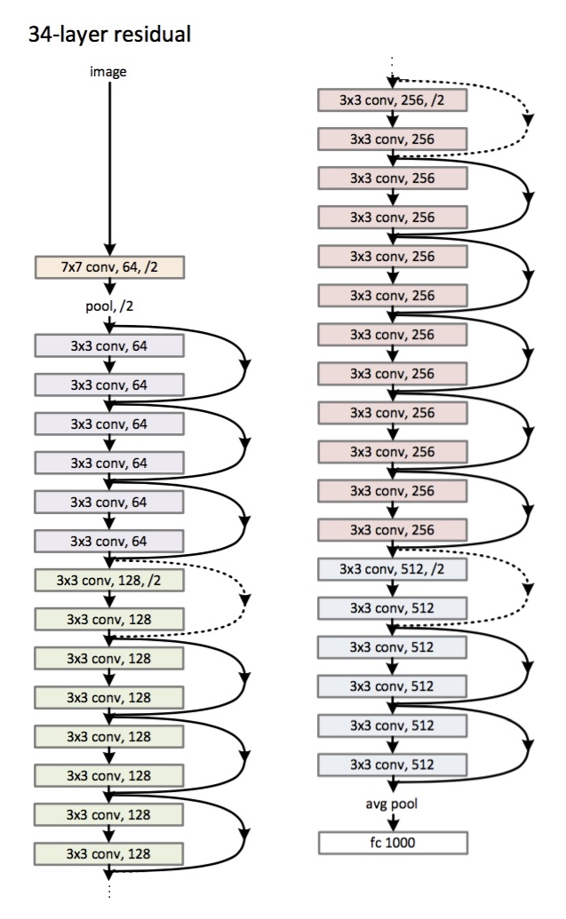
in 2015.
The main innovation is a large number of layers and the so-called residual blocks. These blocks are used to combat the fading gradient problem. The connection between such residual-blocks is called shortcut (arrows in the picture). Now, using these shortcuts, the gradient will reach all the necessary parameters, thereby training the network :)
Important:
- Instead of fully connected layers - average global pooling.
- Residual blocks.
- The network has surpassed humans in recognizing images on the ImageNet dataset (top-5 error).
- Batch-normalization was used for the first time.
- The technique of initializing weights is used (intuition: from a certain initialization of weights, the network converges (learns) faster and better).
- The maximum depth is 152 layers!
A small digression
The problem of fading gradient is relevant for all deep neural networks.
There is also its antagonist - the exploding gradient problem, which is also relevant for all deep neural networks. The bottom line is clear from the name - the gradient becomes too large, which causes NaN (not a number, infinity). The solution is obvious - to limit the value of the gradient, otherwise - to reduce its value (normalize). This technique is called "clipping".
Conclusion
In 2019, an article appeared about a new family of architectures - EfficientNet.
I recommend to follow the latest trends in various tasks and areas related to Machine Learning here . On this resource, you can select a task (for example, image classification) and a dataset (for example, ImageNet) and look at the quality of certain architectures, additional information about them. For example, the FixEfficientNet-L2 grid takes the honorable first place in image classification on the ImageNet dataset (top-1 accuracy).
In the next articles, we'll talk about transfer learning, object detection, segmentation.