Therefore, when an abnormal consumption of resources (CPU, memory, disk, network, ...) occurs on one of the thousands of controlled servers , there is a need to figure out "who is to blame and what to do."
There is a pidstat utility for real-time monitoring of the Linux server resource usage "at the moment" . That is, if the load peaks are periodic, they can be "hatched" right in the console. But we want to analyze this data after the fact , trying to find the process that created the maximum load on resources.
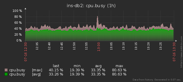
That is, I would like to be able to look at previously collected data various beautiful reports with grouping and detailing on an interval such as these:
In this article, we will consider how all this can be economically located in the database, and how to most effectively collect a report from this data using window functions and GROUPING SETS .
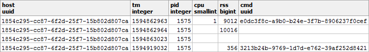
First, let's see what kind of data we can extract if we take "everything to the maximum":
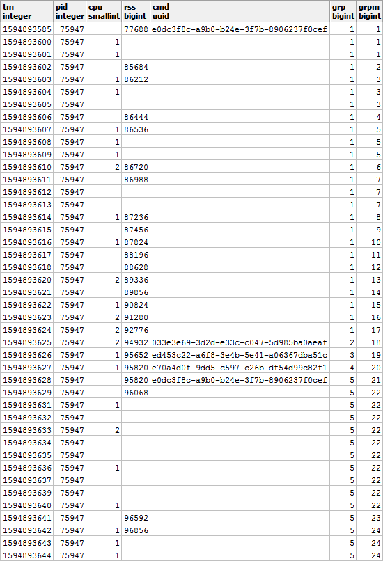
pidstat -rudw -lh 1| Time | UID | PID | % usr | % system | % guest | % CPU | CPU | minflt / s | majflt / s | VSZ | Rss | % MEM | kB_rd / s | kB_wr / s | kB_ccwr / s | cswch / s | nvcswch / s | Command |
| 1594893415 | 0 | 1 | 0.00 | 13.08 | 0.00 | 13.08 | 52 | 0.00 | 0.00 | 197312 | 8512 | 0.00 | 0.00 | 0.00 | 0.00 | 0.00 | 7.48 | / usr / lib / systemd / systemd --switched-root --system --deserialize 21 |
| 1594893415 | 0 | nine | 0.00 | 0.93 | 0.00 | 0.93 | 40 | 0.00 | 0.00 | 0 | 0 | 0.00 | 0.00 | 0.00 | 0.00 | 350.47 | 0.00 | rcu_sched |
| 1594893415 | 0 | thirteen | 0.00 | 0.00 | 0.00 | 0.00 | 1 | 0.00 | 0.00 | 0 | 0 | 0.00 | 0.00 | 0.00 | 0.00 | 1.87 | 0.00 | migration / 11.87 |
All these values are divided into several classes. Some of them change constantly (CPU and disk activity), others rarely (memory allocation), and Command not only rarely changes within the same process, but also regularly repeats on different PIDs.
Base structure
For the sake of simplicity, let's limit ourselves to one metric for each "class" we will save:% CPU, RSS, and Command.
Since we know in advance that Command is repeated regularly, we will simply move it into a separate table-dictionary, where the MD5 hash will act as the UUID key:
CREATE TABLE diccmd(
  cmd
    uuid
      PRIMARY KEY
, data
    varchar
);
And for the data itself, a table of this type is suitable for us:
CREATE TABLE pidstat(
  host
    uuid
, tm
    integer
, pid
    integer
, cpu
    smallint
, rss
    bigint
, cmd
    uuid
);
I would like to draw your attention to the fact that since% CPU always comes to us with an accuracy of 2 decimal places and certainly does not exceed 100.00, then we can easily multiply it by 100 and put it in
smallint. On the one hand, this will save us from the problems of accounting accuracy during operations, on the other hand, it is still better to store only 2 bytes compared to 4 bytes realor 8 bytes double precision.
You can read more about ways to efficiently pack records in PostgreSQL storage in the article "Save a pretty penny on large volumes" , and about increasing the database throughput for writing - in "Writing on sublight: 1 host, 1 day, 1TB" .
"Free" storage of NULLs
To save the performance of the disk subsystem of our database and the size of the database, we will try to represent as much data as possible in the form of NULL - their storage is practically "free", since it takes only a bit in the record header.
More information about the internal mechanics of representing records in PostgreSQL can be found in Nikolai Shaplov's talk at PGConf.Russia 2016 "What's inside it: data storage at a low level . " Slide # 16 is devoted to NULL storage .Let's take a closer look at the types of our data:
- CPU / DSK
Changes constantly, but very often it turns to zero - so it is beneficial to write NULL instead of 0 to the base . - RSS / CMD It
changes quite rarely - therefore we will write NULL instead of repeats within the same PID.
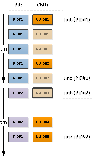
It turns out a picture like this, if you look at it in the context of a specific PID:
It is clear that if our process starts to execute another command, then the value of the used memory will also probably be different from before - so we will agree that when changing CMD, the value of RSS will also be fix regardless of the previous value.
That is , an entry with a filled CMD value has an RSS value as well . Let us remember this moment, it will still be useful to us.
Putting together a beautiful report
Let's now put together a query that will show us the resource consumers of a specific host at a specific time interval.
But let's do it right away with minimal use of resources - similar to the article about SELF JOIN and window functions .
Using incoming parameters
In order not to specify the values of the report parameters (or $ 1 / $ 2) in several places during the SQL query, we will select the CTE from the only json field in which these parameters are located by keys:
--
WITH args AS (
  SELECT
    json_object(
      ARRAY[
        'dtb'
      , extract('epoch' from '2020-07-16 10:00'::timestamp(0)) --  timestamp  integer
      , 'dte'
      , extract('epoch' from '2020-07-16 10:01'::timestamp(0))
      , 'host'
      , 'e828a54d-7e8a-43dd-b213-30c3201a6d8e' --    uuid
      ]::text[]
    )
)
Retrieving raw data
Since we did not invent any complex aggregates, the only way to analyze the data is to read it. For this we need an obvious index:
CREATE INDEX ON pidstat(host, tm);-- ""
, src AS (
SELECT
*
FROM
pidstat
WHERE
host = ((TABLE args) ->> 'host')::uuid AND
tm >= ((TABLE args) ->> 'dtb')::integer AND
tm < ((TABLE args) ->> 'dte')::integer
)
Analysis key grouping
For each found PID, determine the interval of its activity and take the CMD from the first record in this interval.
To do this, we will use uniqueization through
DISTINCT ONand window functions:
--
, pidtm AS (
  SELECT DISTINCT ON(pid)
    host
  , pid
  , cmd
  , min(tm) OVER(w) tmb --
  , max(tm) OVER(w) tme --
  FROM
    src
  WINDOW
    w AS(PARTITION BY pid)
  ORDER BY
    pid
  , tm
)
Process activity limits
Note that relative to the beginning of our interval, the first record that comes across may be either one that already has a filled CMD field (PID # 1 in the picture above), or with NULL, indicating the continuation of the filled “above” value in chronology (PID # 2 ).
Those of the PIDs that were left without CMD as a result of the previous operation began earlier than the beginning of our interval, which means that these "beginnings" need to be found:

Since we know for sure that the next segment of activity begins with a filled CMD value (and there is a filled RSS, which means ), the conditional index will help us here:
CREATE INDEX ON pidstat(host, pid, tm DESC) WHERE cmd IS NOT NULL;-- ""
, precmd AS (
SELECT
t.host
, t.pid
, c.tm
, c.rss
, c.cmd
FROM
pidtm t
, LATERAL(
SELECT
*
FROM
pidstat -- , SELF JOIN
WHERE
(host, pid) = (t.host, t.pid) AND
tm < t.tmb AND
cmd IS NOT NULL --
ORDER BY
tm DESC
LIMIT 1
) c
WHERE
t.cmd IS NULL -- ""
)
If we want (and we want) to know the end time of the segment's activity, then for each PID we will have to use a "two-way" to determine the lower limit.
We have already used a similar technique in PostgreSQL Antipatterns: Navigating the Registry .

--
, pstcmd AS (
  SELECT
    host
  , pid
  , c.tm
  , NULL::bigint rss
  , NULL::uuid cmd
  FROM
    pidtm t
  , LATERAL(
      SELECT
        tm
      FROM
        pidstat
      WHERE
        (host, pid) = (t.host, t.pid) AND
        tm > t.tme AND
        tm < coalesce((
          SELECT
            tm
          FROM
            pidstat
          WHERE
            (host, pid) = (t.host, t.pid) AND
            tm > t.tme AND
            cmd IS NOT NULL
          ORDER BY
            tm
          LIMIT 1
        ), x'7fffffff'::integer) -- MAX_INT4
      ORDER BY
        tm DESC
      LIMIT 1
  ) c
)
JSON conversion of post formats
Note that we selected
precmd/pstcmdonly those fields that affect subsequent lines, and any CPU / DSK that are constantly changing - no. Therefore, the format of records in the original table and these CTEs differs for us. No problem!
- row_to_json - turn each record with fields into a json object
- array_agg - collect all entries in '{...}' :: json []
- array_to_json - convert array-from-JSON to JSON-array '[...]' :: json
- json_populate_recordset - generate a selection of a given structure from a JSON array
Here we use a single callWe glue the found "beginnings" and "ends" into a common heap and add to the original set of records:json_populate_recordsetinstead of a multiple onejson_populate_record, because it is trite much faster.
--
, uni AS (
  TABLE src
UNION ALL
  SELECT
    *
  FROM
    json_populate_recordset( --
      NULL::pidstat
    , (
        SELECT
          array_to_json(array_agg(row_to_json(t))) --
        FROM
          (
            TABLE precmd
          UNION ALL
            TABLE pstcmd
          ) t
      )
    )
)
Filling in null gaps
Let's use the model discussed in the article "SQL HowTo: Build Chains with Window Functions" .First, let's select the "repeat" groups:
--
, grp AS (
  SELECT
    *
  , count(*) FILTER(WHERE cmd IS NOT NULL) OVER(w) grp  --   CMD
  , count(*) FILTER(WHERE rss IS NOT NULL) OVER(w) grpm --   RSS
  FROM
    uni
  WINDOW
    w AS(PARTITION BY pid ORDER BY tm)
)
Moreover, according to CMD and RSS, the groups will be independent of each other, so they may look something like this:
Fill in the gaps in RSS and calculate the duration of each segment in order to correctly take into account the load distribution over time:
--
, rst AS (
  SELECT
    *
  , CASE
      WHEN least(coalesce(lead(tm) OVER(w) - 1, tm), ((TABLE args) ->> 'dte')::integer - 1) >= greatest(tm, ((TABLE args) ->> 'dtb')::integer) THEN
        least(coalesce(lead(tm) OVER(w) - 1, tm), ((TABLE args) ->> 'dte')::integer - 1) - greatest(tm, ((TABLE args) ->> 'dtb')::integer) + 1
    END gln --
  , first_value(rss) OVER(PARTITION BY pid, grpm ORDER BY tm) _rss --    RSS
  FROM
    grp
  WINDOW
    w AS(PARTITION BY pid, grp ORDER BY tm)
)
Multi-grouping with GROUPING SETS
Since we want to see as a result both the summary information for the entire process and its detailing by different segments of activity, we will use grouping by several sets of keys at once using GROUPING SETS :
--
, gs AS (
  SELECT
    pid
  , grp
  , max(grp) qty --     PID
  , (array_agg(cmd ORDER BY tm) FILTER(WHERE cmd IS NOT NULL))[1] cmd -- "   "
  , sum(cpu) cpu
  , avg(_rss)::bigint rss
  , min(tm) tmb
  , max(tm) tme
  , sum(gln) gln
  FROM
    rst
  GROUP BY
    GROUPING SETS((pid, grp), pid)
)
The use case (array_agg(... ORDER BY ..) FILTER(WHERE ...))[1]allows us to get the first non-empty (even if it is not the very first) value from the entire set right when grouping, without additional body movements .The option of obtaining several sections of the target sample at once is very convenient for generating various reports with detailing, so that all detailing data does not need to be rebuilt, but so that it appears in the UI along with the main sample.
Dictionary instead of JOIN
Create a CMD "dictionary" for all found segments:
You can read more about the "mastering" technique in the article "PostgreSQL Antipatterns: Let's Hit a Heavy JOIN with a Dictionary" .
--  CMD
, cmdhs AS (
  SELECT
    json_object(
      array_agg(cmd)::text[]
    , array_agg(data)
    )
  FROM
    diccmd
  WHERE
    cmd = ANY(ARRAY(
      SELECT DISTINCT
        cmd
      FROM
        gs
      WHERE
        cmd IS NOT NULL
    ))
)
And now we use it instead
JOIN, getting the final "beautiful" data:
SELECT
  pid
, grp
, CASE
    WHEN grp IS NOT NULL THEN --  ""
      cmd
  END cmd
, (nullif(cpu::numeric / gln, 0))::numeric(32,2) cpu --  CPU  ""
, nullif(rss, 0) rss
, tmb --
, tme --
, gln --
, CASE
    WHEN grp IS NULL THEN --
      qty
  END cnt
, CASE
    WHEN grp IS NOT NULL THEN
      (TABLE cmdhs) ->> cmd::text --
  END command
FROM
  gs
WHERE
  grp IS NOT NULL OR --   ""
  qty > 1 --
ORDER BY
  pid DESC
, grp NULLS FIRST;
Finally, let's make sure that our entire query turned out to be quite lightweight when executed:
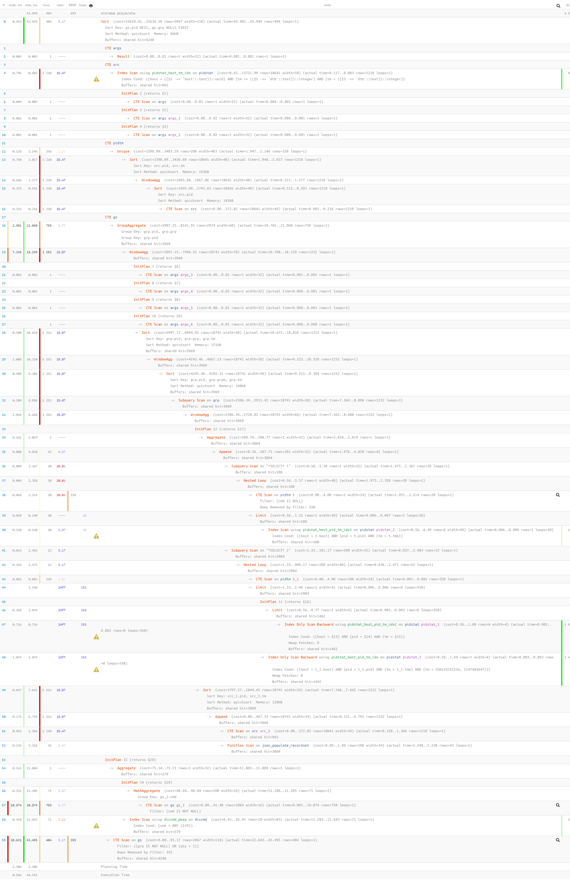
[look at explain.tensor.ru]
Only 44ms and 33MB of data was read!