Hello colleagues! I haven't written on Habr for a hundred years, but now the time has come. This spring, I taught the Advanced ML course at the MADE Big Data Academy from Mail.ru Group; It seems that the listeners liked it, and now I was asked to write not so much an advertising post as an educational post about one of the topics of my course. The choice was close to the obvious: as an example of a complex probabilistic model, we discussed an extremely relevant (seemingly ... but more on that later) epidemiological SIR model that models the spread of diseases in a population. It has everything: approximate inference through Markov Monte Carlo methods, and hidden Markov models with the Viterbi stochastic algorithm, and even presence-only data.
With this topic, only one small difficulty came out: I began to write about what I actually told and showed at the lecture ... and somehow quickly and imperceptibly twenty pages of text (well, with pictures and code) accumulated, which is still not was finished and was not self-contained at all. And if you tell everything in such a way that it is clear from "zero" (not from absolute zero, of course), then you could write a hundred pages. So someday I will definitely write them, but for now I present to your attention the first part of the description of the SIR model, in which we can only pose a problem and describe the model from its generating side - and if the respected public has an interest, then it will be possible proceed.
SIR model: problem statement
I love my friends and they love me,
We're just as close as we can be.
And just because we really care,
Whatever we get, we share!
Tom Lehrer. I Got It From Agnes
So let's figure it out. Informally, the basic assumptions of the SIR model are as follows:
- there is a certain population of people in which some terrible virus can walk;
- initially, the virus enters the population one way or another (for example, the first sick person appears), and then people become infected from each other;
- SIR , :
○ Susceptible ( , , .. ),
○ Infected ( )
○ Recovered ().
For simplicity, we will assume that those who have been ill always develop immunity, and they are excluded from the cycle of the virus in nature. Accordingly, transitions between these states can only be from left to right: Susceptible → Infected → Recovered.
The task is, in fact, to train this model, that is, to understand something about the parameters of the infection process from the data. It is easy to understand how the data looks like - it is simply the number of registered infected at each moment in time, which we will denote by the vector... For example, when I gave my homework in the course on coronavirus (it was, however, about other models), the data for Russia looked like this:
[2,2,2,2,3,4,6,8,10,10,10,10,15,20,25,30,45,59,63,93,114,147,199,253,306,438,438,495,658,840,1036,1264,1534,1836,2337,2777,3548,4149,4731,5389,6343,7497,8672]But what the parameters of this model are, how they interface with each other and how to train them, especially on such a tiny dataset, is a more serious question.
In general, I will follow the general outline of the work ( Fintzi et al., 2016 ), which builds MCMC algorithms for the SIR, SEIR models and some of their variants. But in comparison with ( Fintzi et al., 2016 ), I will greatly simplify both the model and its presentation. The main simplification is that instead of continuous time, which is considered in the original work, we will consider discrete time, that is, instead of a continuous process that at some point generates events of the form "infected" and "recovered", we will consider that people go through a set of discrete points in time... This simplification will allow us, firstly, to get rid of many technical difficulties, and secondly, to switch from the Metropolis-Hastings algorithm in general to the Gibbs sampling algorithm, that is, not to calculate the Metropolis ratio, as it is necessary to do in ( Fintzi et al., 2016 ). If you do not understand what I just said, do not worry: we will not need this today, and if there are next parts, I will explain everything there.
We will denote the states of the SIR model by S, I, and R, respectively, and the state of a person at the moment - across ... At the same time, we will immediately introduce variables for the total number of patients who have not yet become ill.sick and recovered at the moment ... Total man we will haveso for anyone will be executed ... And, as I wrote above,of them are registered (tested) sick people.
The unknown parameters of the model arewhere:
- - the initial distribution of cases; in other words, for each ; in our simplified model, we will not train, but we will simply record 1-2 cases at the first moment of time;
- - the probability of finding an infected person in the general population, that is, the probability that a person in the moment when , will be detected by testing and enrolled in the data ; in other words, for each sick person, we flip a coin to determine whether testing will find it or not, so the current item is has a binomial distribution with parameters and :
- - the probability for the sick person to recover in one time step, that is, the probability of transition from the state in state ;
AND - This is the most interesting parameter showing the probability of infection in one count of time from one infected person . This means that in the model we assume that all people in the population “communicate” with each other (“communication” here means contact sufficient for the transmission of the disease; coronavirus is transmitted mainly by airborne droplets, but, of course, it is possible to model and the spread of any other disease; see, for example, the epigraph), and the likelihood of becoming infected depends on how many are now infected, that is, on what is... We will assume the simplest model, in which the probability of infection from one infected person is, and all these events are independent, which means that the probability of staying healthy is
These assumptions actually have a lot to discuss. The most surprising thing here, in my personal opinion, is the binomial distribution for... Tossing a coin with the probability of detecting an infected person is absolutely normal, but it is not very realistic that we toss this coin again at every step, that is, we can “forget” an already detected infected person. As a result, the SIR model can (and often does) produce a completely non-monotonic sequence; this is strange, but it does not seem to have much effect on the result, and it would be much more difficult to model this process more realistically.
In addition, it is obvious that this model is intended for a closed population, where everyone "communicates" with everyone, so it makes no sense to launch it, say, for Russia with the parameter N of one hundred million or for Moscow with the parameter ten million (and computationally will not work). An important direction of extensions and continuation of SIR-models is devoted to this: how to add a more realistic graph of interactions and possible infections; we will probably talk about this in the last, final post.
But with all these simplifications, now, using the above parameters, we can write out the probability matrix of transition between states. These probabilities (more precisely, specifically the probability of being infected) depend on the general statistics of the population. Let's designate the vector of states of all people except, across , and extend the same notation to all other variables; eg, Is the number of infected at a time , not to mention ... Then, for the probabilities of transition from at we get
and in all other cases
The same can be written more clearly in the form of a transition probability matrix (the order of rows and columns is natural, SIR):
To a reader familiar with Markov chains and Markov models, it may seem that this is just a hidden Markov model: there is a hidden state, there is a clear distribution of observables for each hidden state, the transitions are really Markov, that is, the next hidden state depends only on the previous one ... But there is , as they say, there is one caveat: the transition probabilities cannot be considered constant, they change with the change, and this is an extremely important aspect of the model that cannot be thrown away.
Therefore, inference in this model suddenly becomes much more difficult than in the usual hidden Markov model (although there is also not always such a gift). However, although the conclusion is more complicated, it is still subject to the human mind - in the next installations (if any) I will tell you about this. And for today, almost enough is enough - now let's relax a little and try to play with this model for the time being in a generative sense.
Data Generation Example
As a great connoisseur and expert, an
introvert went into quarantine.
***
“I couldn't work at home,” the
bee tried to explain to the worms.
***
Kaganov died joking merrily.
Of course, I'm very sorry for him, though ...
Leonid Kaganov. Quarantines
If the parameters of the model are known, and you just need to generate a trajectory of how the spread of the disease in the population would develop, there is nothing complicated in SIR. The code below generates an example of a population according to our model; states I coded as, , ... As I warned, for simplicity I will assume that at the moment in time there is exactly one sick person in the population, and then it goes on.
def sample_population(N, T, true_rho, true_beta, true_mu):
    true_log1mbeta = np.log(1 - true_beta)

    cur_states = np.zeros(N)
    cur_states[:1] = 1
    cur_I, test_y, true_statistics = 1, [1], [[N-1, 1, 0]]

    for t in range(T):
        logprob_stay_healthy = cur_I * true_log1mbeta
        for i in range(N):
            if cur_states[i] == 0 and np.random.rand() < -np.expm1(logprob_stay_healthy):
                cur_states[i] = 1
            elif cur_states[i] == 1 and np.random.rand() < true_mu:
                cur_states[i] = 2

        cur_I = np.sum(cur_states == 1)
        test_y.append( np.random.binomial( cur_I, true_rho ) )
        true_statistics.append([np.sum(cur_states == 0), np.sum(cur_states == 1), np.sum(cur_states == 2)])

    return test_y, np.array(true_statistics).T

N, T, true_rho, true_beta, true_mu = 100, 20, 0.1, 0.05, 0.1
test_y, true_statistics = sample_population(N, T, true_rho, true_beta, true_mu)
This code gives out not only the actual data but also "true" statistics , , so they can be visualized. Let's do it; for parameters, , , , you can get something like this:
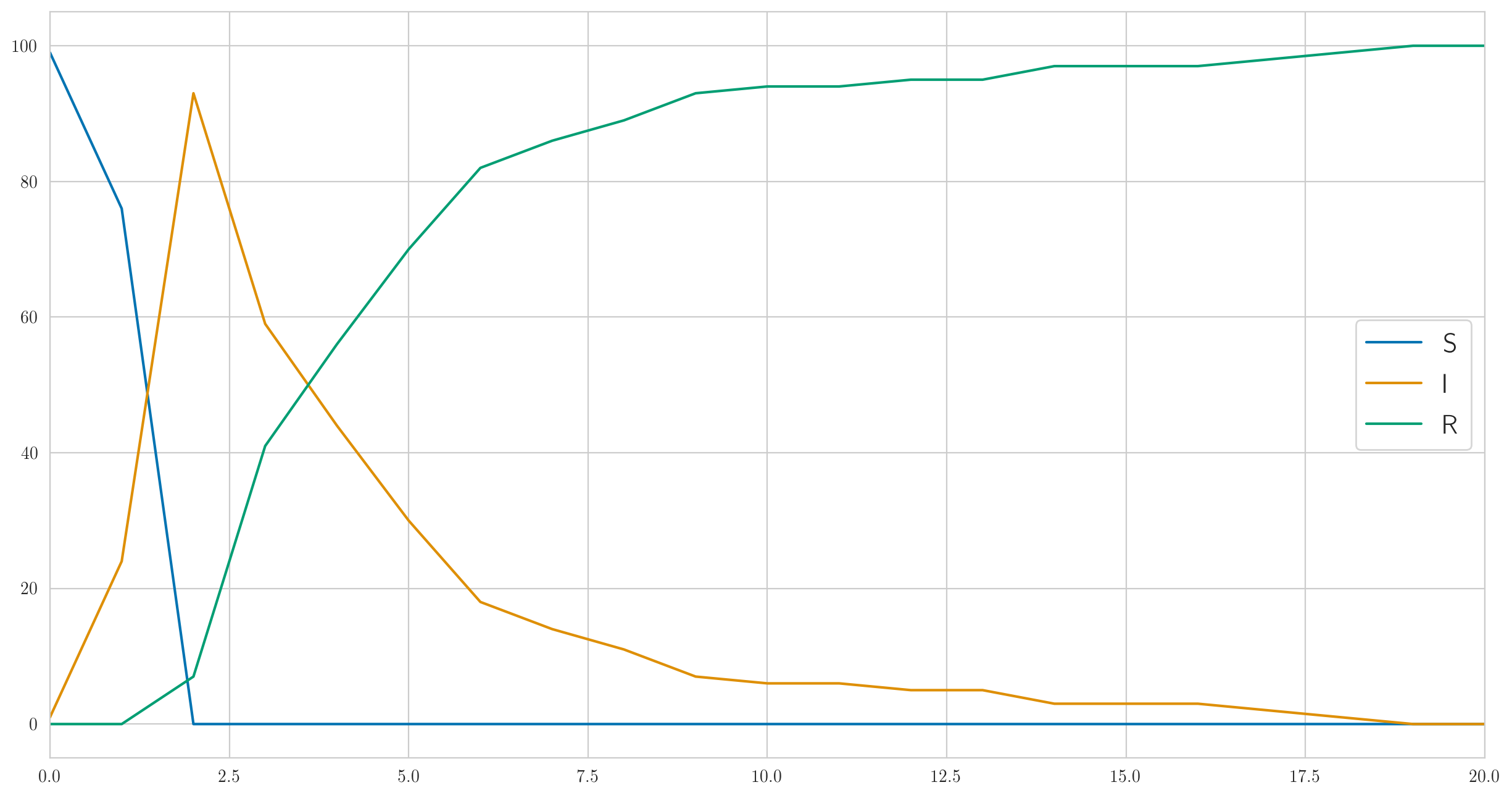
As you can see, in this example, everyone gets sick very quickly, and then slowly begins to get better. And the actual observed data on the sick look like this:
[1 6 13 6 6 4 1 0 0 1 0 1 2 0 0 0 0 0 1 0 0]
Note that, as we discussed above, there is no monotony here.
But this is certainly not the only possible behavior. I chose the parameters above so that the infection was fast enough and the disease almost immediately covered all one hundred people in our test population. And if you do smaller, for example , then the infection will go much slower, and not even everyone will have time to get sick before the last sick person recovers and will not stay. Something like this:
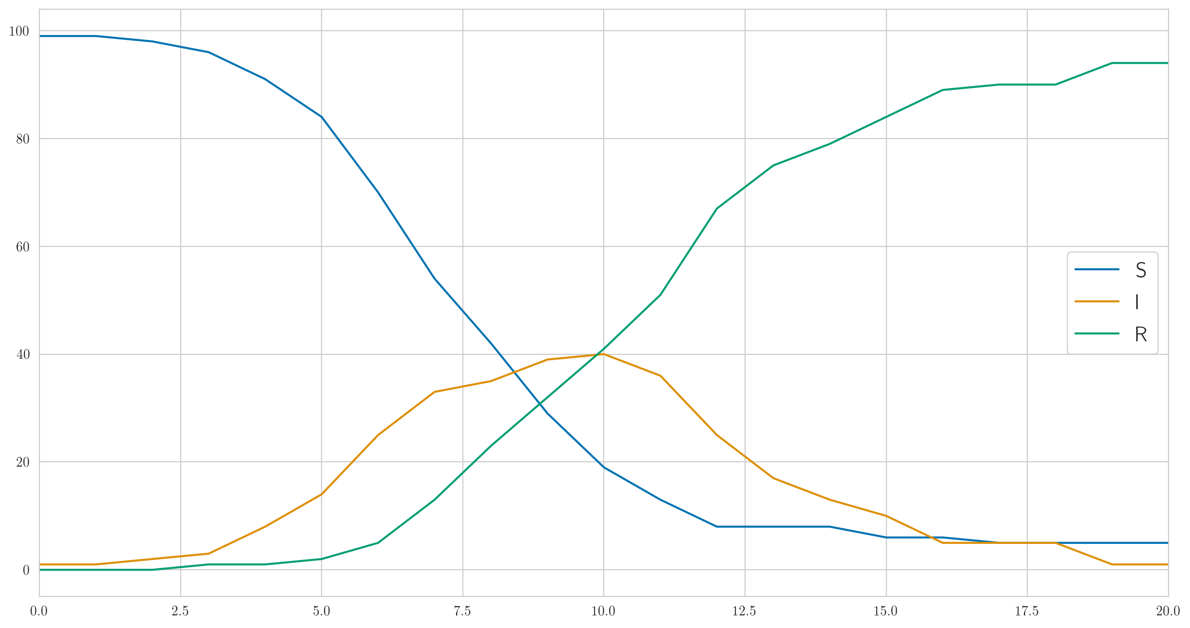
And the number of detected cases is also completely different:
[1 0 0 0 0 1 2 2 3 1 1 9 3 1 3 1 0 1 0 0 0]
It is possible to "strangle" the disease even more; for example let's leavebut put , that is, at each time interval, each sick person has a chance to recover by 0.5 (in the end, this is logical: either he will recover or not). Then only 50-60 out of 100 people will get sick with the terrible virus; curves can look like this:

[1 0 0 1 3 2 1 1 0 3 0 0 0 0 0 1 0 0 0 0 0]
But the overall picture, of course, in any case looks about the same: first exponential growth, and then the exit to saturation; the only difference is whether the last carrier has time to recover before everyone is rebooted.
Well, it's time to sum up the interim results. Today we have seen what one of the simplest epidemiological models looks like. Despite a bunch of oversimplifying assumptions, the SIR model is still very useful even in this form; the fact is that most of its extensions are fairly straightforward and do not change the general essence of the matter. Therefore, if we continue, in the next series I will talk about how to train an SIR model; however, this will entail so many interesting things that it probably won't fit in one post either. Until next time!