Introduction
The architecture of the Convolutional Neural Network (CNN) RetinaNet consists of 4 main parts, each of which has its own purpose:
a) Backbone - the main (basic) network used to extract features from the input image. This part of the network is variable and may include classification neural networks such as ResNet, VGG, EfficientNet and others;
b) Feature Pyramid Net (FPN) - a convolutional neural network, built in the form of a pyramid, serving to combine the advantages of feature maps of the lower and upper levels of the network, the former have high resolution, but low semantic, generalizing ability; the latter, on the contrary;
c) Classification Subnet - a subnet that extracts information about object classes from FPN, solving the classification problem;
d) Regression Subnet - a subnet that extracts information about the coordinates of objects in the image from FPN, solving the regression problem.
In fig. 1 shows the architecture of the RetinaNet with the ResNet neural network as the backbone.
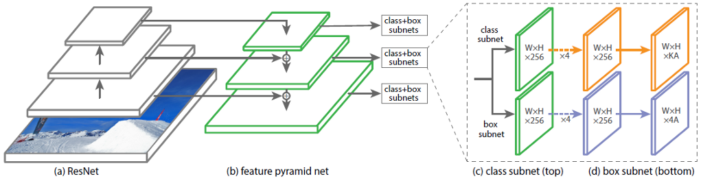
Figure 1 - RetinaNet architecture with a ResNet backbone
Let's analyze in detail each of the RetinaNet parts shown in Fig. 1.
Backbone is part of the RetinaNet network
Considering that the part of the RetinaNet architecture that accepts an image as input and highlights important features is variable and the information extracted from this part will be processed in the next stages, it is important to choose a suitable backbone network for the best results.
Recent research on CNN optimization has led to the development of classification models that outperform all previously developed architectures with the best accuracy rates on the ImageNet dataset, while improving efficiency by 10 times. These networks were named EfficientNet-B (0-7). The indicators of the family of new networks are shown in Fig. 2.
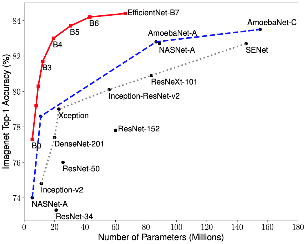
Figure 2 - Graph of the dependence of the highest accuracy indicator on the number of network weights for various architectures
The pyramid of signs
The Feature Pyramid Network consists of three main parts: bottom-up pathway, top-down pathway, and lateral connections.
The upward path is a kind of hierarchical "pyramid" - a sequence of convolutional layers with decreasing dimension, in our case - a backbone network. The upper layers of the convolutional network have more semantic meaning, but lower resolution, and the lower ones, on the contrary (Fig. 3). Bottom-up pathway has a vulnerability in feature extraction - the loss of important information about an object, for example, due to noise of a small but significant object in the background, since by the end of the network the information is highly compressed and generalized.
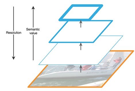
Figure 3 - Features of feature maps at different levels of the neural network
The descending path is also a "pyramid". The feature maps of the upper layer of this pyramid have the size of the feature maps of the upper layer of the bottom-up of the pyramid and are doubled by the nearest neighbor method (Fig. 4) downward.
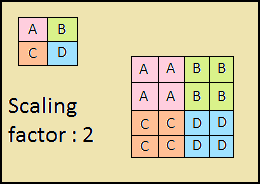
Figure 4 - Increasing the image resolution by the nearest neighbor method
Thus, in the top-down network, each feature map of the overlying layer is increased to the size of the underlying map. In addition, side connections are present in FPN, which means that feature maps of the corresponding bottom-up and top-down layers of the pyramids are added element by element, and the maps from the bottom-up are folded 1 * 1. This process is shown schematically in Fig. 5.
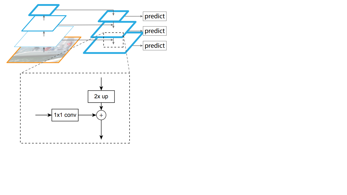
Figure 5 - The structure of the pyramid of signs
Lateral connections solve the problem of attenuation of important signals in the process of passing through the layers, combining semantically important information received at the end of the first pyramid and more detailed information obtained earlier in it.
Further, each of the resulting layers in the top-down pyramid is processed by two subnets.
Classification and regression subnets
The third part of the RetinaNet architecture is two subnets: classification and regression (Figure 6). Each of these subnets forms at the output a response about the class of the object and its location on the image. Let's consider how each of them works.
Figure 6 - RetinaNet subnets
The difference in the principles of the considered blocks (subnets) does not differ until the last layer. Each of them consists of 4 layers of convolutional networks. 256 feature maps are formed in the layer. On the fifth layer, the number of feature maps changes: the regression subnet has 4 * A feature maps, the classification subnet has K * A feature maps, where A is the number of anchor frames (detailed description of anchor frames in the next subsection), K is the number of object classes.
In the last, sixth, layer, each feature map is transformed into a set of vectors. The regression model at the output has for each anchor box a vector of 4 values indicating the offset of the ground-truth box relative to the anchor box. The classification model has a one-hot vector of length K at the output for each anchor frame, in which the index with the value 1 corresponds to the class number that the neural network assigned to the object.
Anchor frames
In the last section, the term anchor frames was used. Anchor box is a hyperparameter of neural networks-detectors, a predefined bounding rectangle with respect to which the network operates.
Let's say the network has a 3 * 3 feature map at the output. In RetinaNet, each cell has 9 anchor boxes, each with a different size and aspect ratio (Figure 7). During training, anchor frames are matched to each target frame. If their IoU indicator has a value of 0.5, then the anchor frame is assigned as the target, if the value is less than 0.4, then it is considered the background, in other cases the anchor frame will be ignored for training. The classification network is trained relative to the assignment (object class or background), the regression network is trained relative to the coordinates of the anchor frame (it is important to note that the error is calculated relative to the anchor frame, but not the target frame).
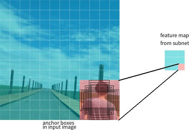
Figure 7 - Anchor frames for one cell of the feature map with a size of 3 * 3
Loss functions
RetinaNet losses are composite, they are composed of two values: the regression or localization error (denoted as Lloc below) and the classification error (denoted as Lcls below). The general loss function can be written as:
Where λ is a hyperparameter that controls the balance between the two losses.
Let's consider in more detail the calculation of each of the losses.
As described earlier, each target frame is assigned an anchor. Let's denote these pairs as (Ai, Gi) i = 1, ... N, where A represents the anchor, G is the target frame, and N is the number of matched pairs.
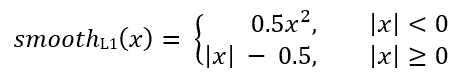
For each anchor, the regression network predicts 4 numbers, which can be denoted as Pi = (Pix, Piy, Piw, Pih). The first two pairs represent the predicted difference between the coordinates of the centers of the anchor Ai and the target frame Gi, and the last two represent the predicted difference between their width and height. Accordingly, for each target frame, Ti is calculated as the difference between the anchor and target frames:
Where smoothL1 (x) is defined by the formula below:
RetinaNet classification problem loss is calculated using the Focal loss function.
where K is the number of classes, yi is the target value of the class, p is the probability of predicting the i-th class, γ is the focus parameter, α is the bias coefficient. This feature is an advanced cross entropy feature. The difference lies in the addition of the parameter γ∈ (0, + ∞), which solves the problem of class imbalance. During training, most of the objects processed by the classifier are the background, which is a separate class. Therefore, a problem may arise when the neural network learns to determine the background better than other objects. The addition of a new parameter solved this problem by reducing the error value for easily classified objects. The graphs of the focal and cross entropy functions are shown in Fig. 8.
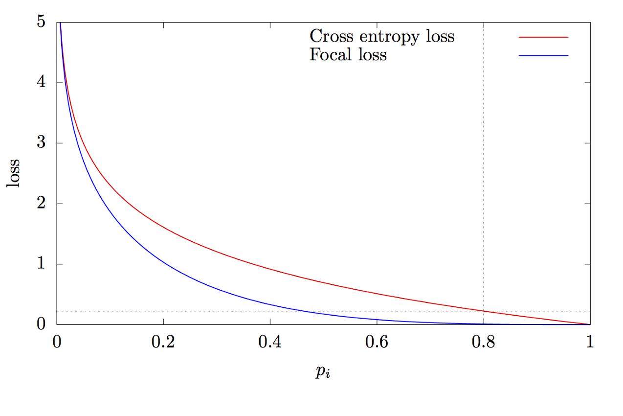
Figure 8 - Graphs of focal and cross entropy functions
Thanks for reading this article!
List of sources:
- Tan M., Le Q. V. EfficientNet: Rethinking Model Scaling for Convolutional Neural Networks. 2019. URL: arxiv.org/abs/1905.11946
- Zeng N. RetinaNet Explained and Demystified [ ]. 2018 URL: blog.zenggyu.com/en/post/2018-12-05/retinanet-explained-and-demystified
- Review: RetinaNet — Focal Loss (Object Detection) [ ]. 2019 URL: towardsdatascience.com/review-retinanet-focal-loss-object-detection-38fba6afabe4
- Tsung-Yi Lin Focal Loss for Dense Object Detection. 2017. URL: arxiv.org/abs/1708.02002
- The intuition behind RetinaNet [ ]. 2018 URL: medium.com/@14prakash/the-intuition-behind-retinanet-eb636755607d