Bayesian Networks with Python - Explained with Examples
Due to limited information (especially in native Russian) and resources of work, Bayesian networks are surrounded by a number of problems. And one could sleep well if they weren't implemented in most of the advanced technologies of the era, such as artificial intelligence and machine learning.
Based on this fact, this article is completely devoted to the work of Bayesian networks and how they themselves can not form problems, but be applied in solving them, even if the problems being solved are extremely confusing.
Article structure
- What is a Bayesian Network?
- What are directed acyclic graphs?
- What math lies in Bayesian networks
- An example reflecting the idea of a Bayesian network
- The essence of the Bayesian network
- Bayesian network in Python
- Application of Bayesian networks
Let's go.
What is a Bayesian Network?
Bayesian networks fall into the category of probabilistic graphical models (GPM). VGMs are used to calculate variability for application in concepts of probability.
The common name for Bayesian networks is Deep Networks. They are used to model directed acyclic graphs.
What are directed acyclic graphs?
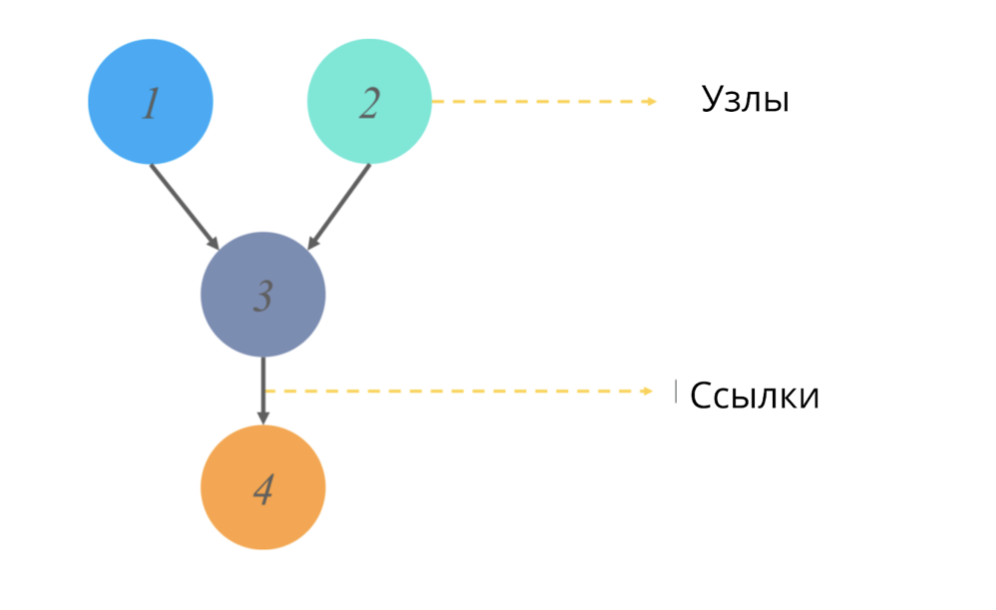
A directed acyclic graph (like any graph in statistics) is a structure of nodes and links, where nodes are responsible for some values, and links reflect relationships between nodes.
Acyclic == not having directed cycles. In the context of graphs, this adjective means that starting a path from one point, we do not go through the entire diagram of the graph, but only part of it. (That is, for example, if we start from node 2 in the picture, we will definitely not get to node 1).
What do these graphs simulate and what output value do they give?
Models of uncertain directed graphs are also based on a change in the probabilistic origin of an event for each of the random values. A conditional probability table is applicable to represent and interpret each value and thus we can simulate the branching of the probability of sequential events.
All OK. I also got confused at first. For a better understanding, let's analyze the mathematical component of Bayesian networks.
Bayesian Network Mathematics
As already mentioned in the definition, Bayesian Networks are based on the theory of probability, therefore, before starting to work with Bayesian networks, two questions must be dealt with:
What is conditional probability?
What is the joint mean probability distribution?
Conditional probability The
conditional probability of some X event is the numerical value of the probability that the event X will occur, provided that some event Y has already occurred.
The standard probability formula for one value (not given in the article): P (X) = n (x) / N, where n are the events under investigation, and N are all possible events.
For two values, the following formulas apply:
If X and Y are dependent events:
P (X or Y) = P (X ⋂ Y) / P (Y), the intersection of the probability of X and Y / on the probability Y. (The sign “” in the numerator means the intersection of probabilities)
If events X and Y are independent:
P (X or Y) = P (X), that is, the occurrence of the events under study is equally likely to each other.
Joint probability
Joint probability is the definition of a statistical measure for two or more events occurring at the same time. That is, events X, Y and, let's say C occur together and we reflect their cumulative probability using the value P (X ⋂ Y ⋂ C).
How does this work in Bayesian networks? Let's look at an example.
An example that reflects the essence of the Bayesian network
Let's say we need to model the probability of getting one of the grades of a student's grade on an exam.
The score is made up of:
- Exam difficulty level (e): discrete variable with two gradations (hard, easy)
- Student IQ: discrete variable with two gradations (low, high)
The resulting assessment value will be used as a predictor (predictive value) of the probability of a student or female student entering the university.
However, the IQ variable will also affect admission to admission.
We represent all values using a directed acyclic graph and a conditional probability distribution table.
Using this representation, we can calculate some cumulative probability, formed from the product of the conditional probabilities of five variables.
Cumulative probability:
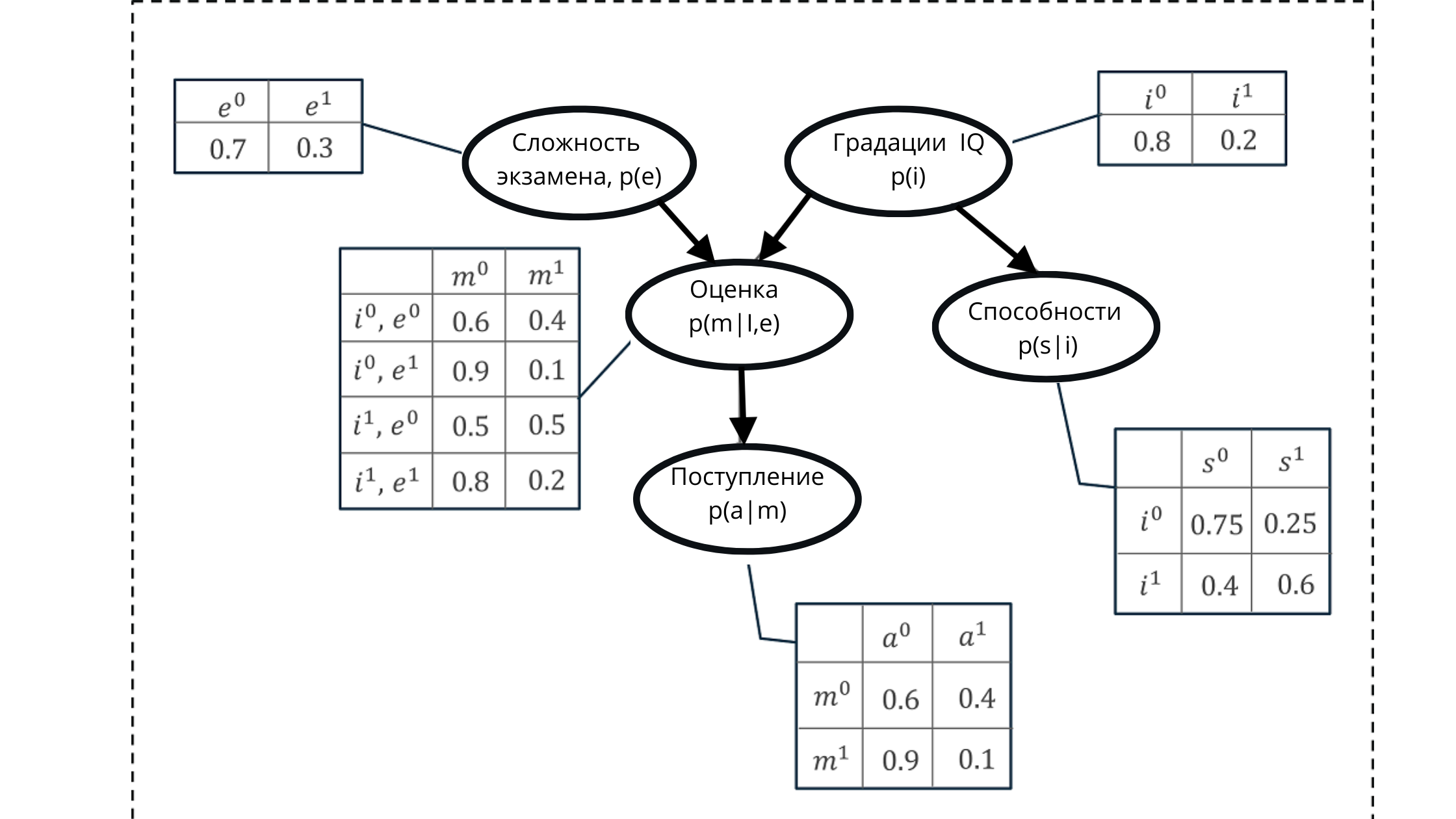
In the illustration:
p (e) is the probability distribution for the grades of the exam variable (affects the grade p (m | i, e)))
p (i) is the probability distribution for the grades of the IQ variable (affects the grade p (m | i, e )))
p (m | i, e) - probability distribution for grade grades, based on IQ level and exam difficulty (depends on p (i) and p (e))
p (s | i) - probability coefficients for student abilities , based on the level of his IQ (depends on the variable IQ p (i))
p (a | m) is the probability of a student's enrollment in the university, based on his estimates p (m | i, e)
Here, I recall that the property of an acyclic graph is a reflection relationship. In the figure, we can clearly see how parent nodes affect children and how children depend on parent.
Hence the formulation of the set of values generated using Bayesian networks emerges.
The essence of the Bayesian Network
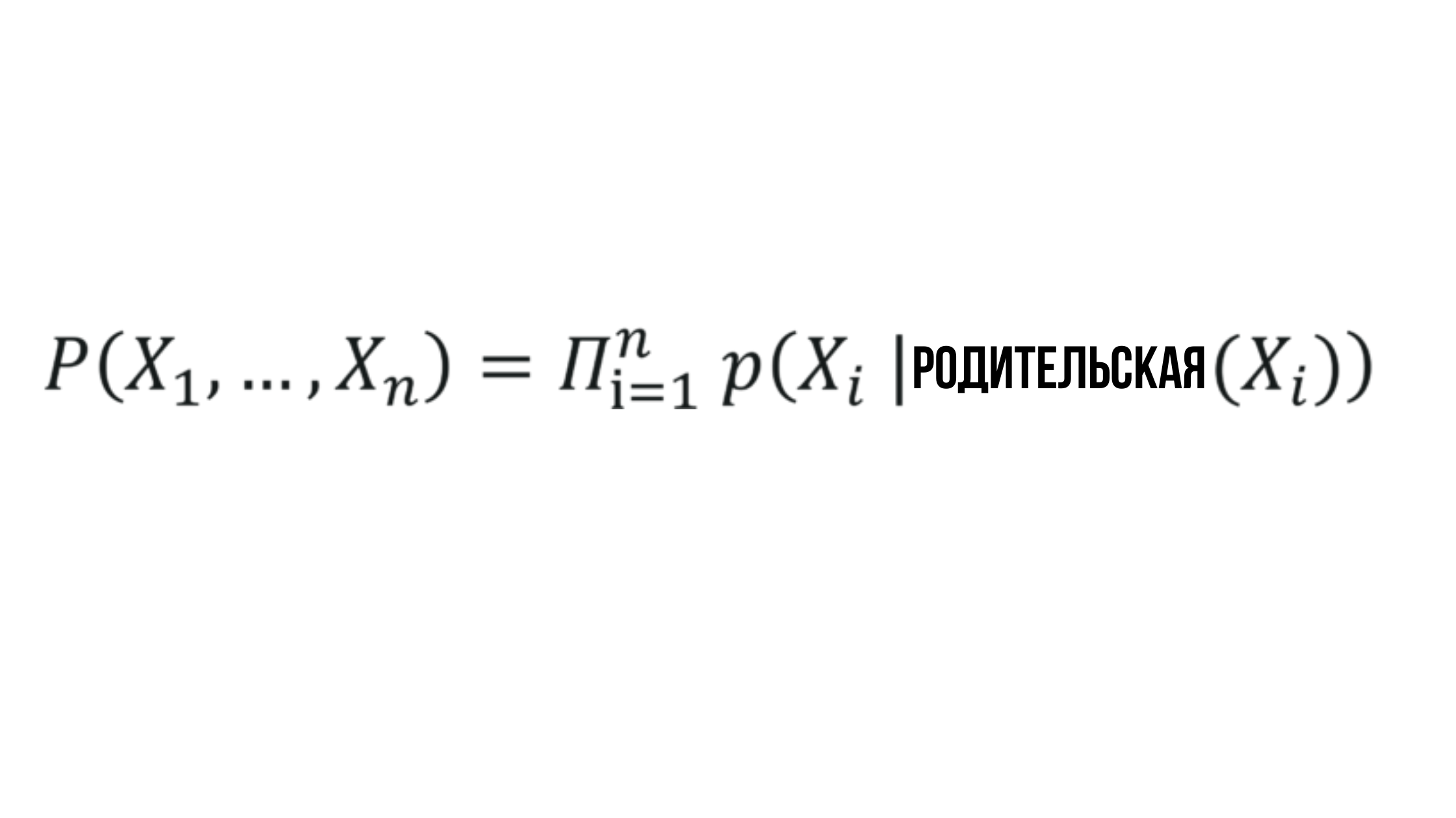
Where the probability X_i depends on the probability of the corresponding parent node and can be represented by any random value.
Sounds simple, and rightly so - Bayesian networks are one of the simplest methods used in descriptive analysis, predictive modeling, and more.
Bayesian Network in Python
Let's look at applying a Bayesian network to a problem called the Monty Hall paradox.
The bottom line: Imagine that you are a participant in the update format of the "Field of Miracles" game. The drum is no longer spinning - now you should not apply your F, but play with p.
There are three doors in front of you, behind which one car is equally likely to be located. The doors, behind which there is no car, will lead you to the goats.
After choosing, the leader of the remaining opens the one that leads to the goat (for example, you chose door 1, which means that the leader opens either door 2 or 3) and invites you to change your choice.
Question: what to do?
Solution: initially the probability of choosing a door with a car = 33%, and with a goat = 66%.
- If you hit 33%, changing the door leads to a loss => chance of winning == 33%
- If you hit 66% the change leads to a win => probability of winning == 66%
From the point of view of mathematical logic, changing the door in aggregate leads to a win in 66% of percent, and to a loss in 33%. Therefore, the correct strategy is to change the door.
But we are talking about the network here, and there can be a lot of doors, so we will transfer the solution to the model.
Let's construct a directed acyclic graph with three nodes:
- Prize door (always with a car)
- Selectable door (either with a car or with a goat)
- Openable door in event 1 (always with a goat)
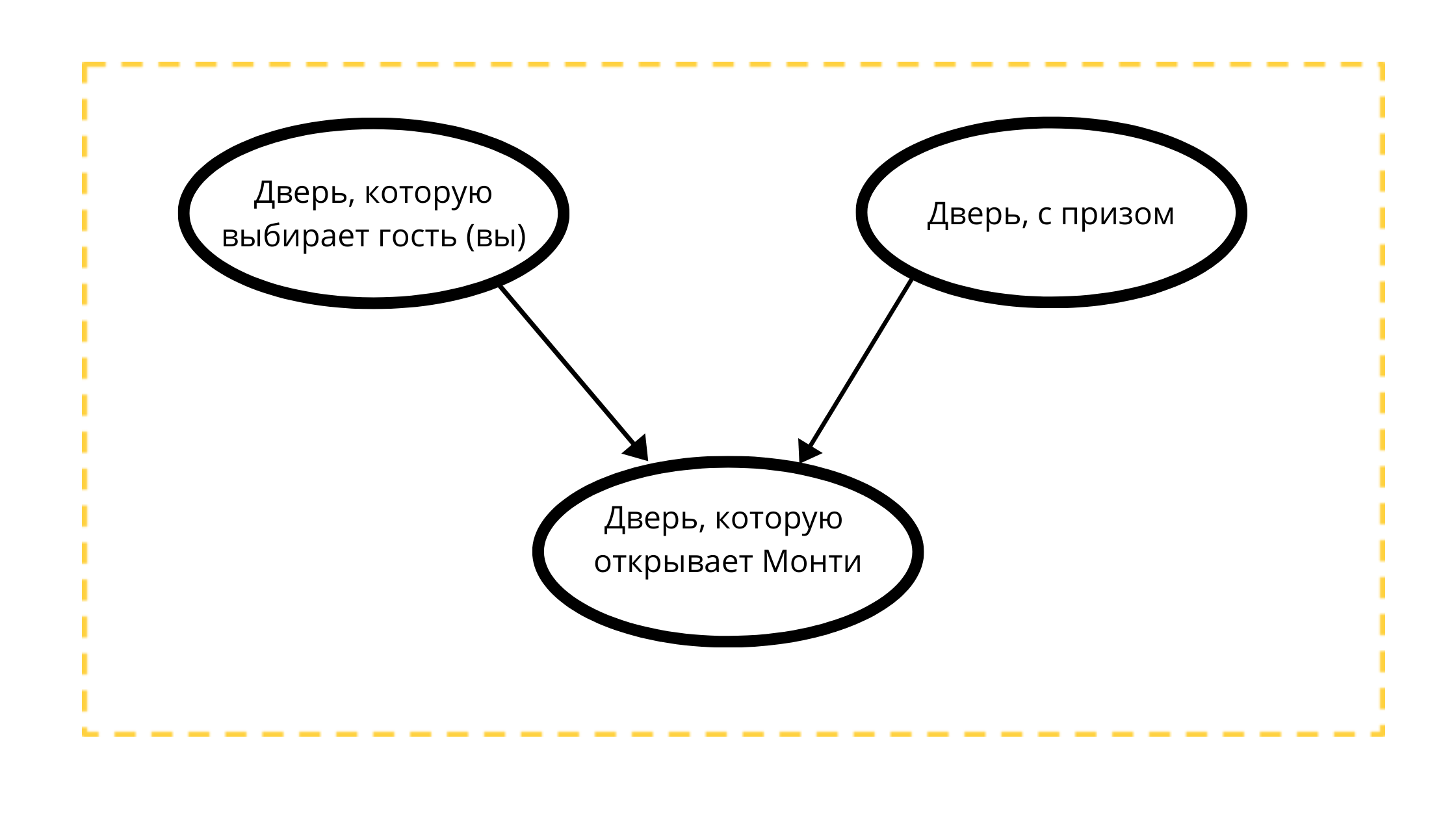
Reading the Count:
The door Monty will open is strictly influenced by two variables:
- The door chosen by the guest (you) tk Monti 100% will NOT open your choice
- A door with a prize, maybe Monty always opens a non-prize door.
According to the mathematical conditions of the classical example, the prize can be equally likely located behind any of the doors, just as you can equally likely choose any door.
#
import math
from pomegranate import *

#    "  " (   3)
guest =DiscreteDistribution( { 'A': 1./3, 'B': 1./3, 'C': 1./3 } )

#    "   " (    )
prize =DiscreteDistribution( { 'A': 1./3, 'B': 1./3, 'C': 1./3 } )

#  ,       ,
#
monty =ConditionalProbabilityTable(
[[ 'A', 'A', 'A', 0.0 ],
[ 'A', 'A', 'B', 0.5 ],
[ 'A', 'A', 'C', 0.5 ],
[ 'A', 'B', 'A', 0.0 ],
[ 'A', 'B', 'B', 0.0 ],
[ 'A', 'B', 'C', 1.0 ],
[ 'A', 'C', 'A', 0.0 ],
[ 'A', 'C', 'B', 1.0 ],
[ 'A', 'C', 'C', 0.0 ],
[ 'B', 'A', 'A', 0.0 ],
[ 'B', 'A', 'B', 0.0 ],
[ 'B', 'A', 'C', 1.0 ],
[ 'B', 'B', 'A', 0.5 ],
[ 'B', 'B', 'B', 0.0 ],
[ 'B', 'B', 'C', 0.5 ],
[ 'B', 'C', 'A', 1.0 ],
[ 'B', 'C', 'B', 0.0 ],
[ 'B', 'C', 'C', 0.0 ],
[ 'C', 'A', 'A', 0.0 ],
[ 'C', 'A', 'B', 1.0 ],
[ 'C', 'A', 'C', 0.0 ],
[ 'C', 'B', 'A', 1.0 ],
[ 'C', 'B', 'B', 0.0 ],
[ 'C', 'B', 'C', 0.0 ],
[ 'C', 'C', 'A', 0.5 ],
[ 'C', 'C', 'B', 0.5 ],
[ 'C', 'C', 'C', 0.0 ]], [guest, prize] )

d1 = State( guest, name="guest" )
d2 = State( prize, name="prize" )
d3 = State( monty, name="monty" )

#
network = BayesianNetwork( "Solving the Monty Hall Problem With Bayesian Networks" )
network.add_states(d1, d2, d3)
network.add_edge(d1, d3)
network.add_edge(d2, d3)
network.bake()
In the snippet the values are:
- A - the door chosen by the guest
- B - prize door
- C - door chosen by Monty
On the fragment, we calculate the probability value for each of the nodes of the graph. The top two nodes obey in our example an equal probability distribution, and the third reflects the dependent distribution. Therefore, in order not to lose value, the probabilities of each of the possible combinations of the game are calculated for .
Having prepared the data, we create a Bayesian network.
It is important to note here that one of the properties of such a network is to reveal the influence of hidden variables on observables. At the same time, neither hidden nor observable variables need to be specified or determined in advance - the model itself examines the influence of hidden variables and will do this the more accurately, the more variables it receives.
Let's start making predictions.
beliefs = network.predict_proba({ 'guest' : 'A' })
beliefs = map(str, beliefs)
print("n".join( "{}t{}".format( state.name, belief ) for state, belief in zip( network.states, beliefs ) ))

guest A
prize {
"class" :"Distribution",
"dtype" :"str",
"name" :"DiscreteDistribution",
"parameters" :[
{
"A" :0.3333333333333333,
"B" :0.3333333333333333,
"C" :0.3333333333333333
}
],
}

monty {
"class" :"Distribution",
"dtype" :"str",
"name" :"DiscreteDistribution",
"parameters" :[
{
"C" :0.49999999999999983,
"A" :0.0,
"B" :0.49999999999999983
}
],
}
Let's analyze the fragment using the example of variable A.
Suppose the guest chose it (A).
The event “there is a prize behind the door” at the stage of choosing a door by a guest has a probability distribution == ⅓ (since each door can be equally likely to be a prize).
Next, add the value of the probabilities of the door being the prize at the stage when the door is chosen by Monty. Since we do not know if the prize door was excluded by our own (guest) choice at step 1, the probability of the door being a prize at this stage is 50/50
beliefs = network.predict_proba({'guest' : 'A', 'monty' : 'B'})
print("n".join( "{}t{}".format( state.name, str(belief) ) for state, belief in zip( network.states, beliefs )))

guest A
prize {
"class" :"Distribution",
"dtype" :"str",
"name" :"DiscreteDistribution",
"parameters" :[
{
"A" :0.3333333333333334,
"B" :0.0,
"C" :0.6666666666666664
}
],
}
monty B
In this step, we will modify the input values for our network. Now it works with the probability distribution obtained in steps 1 and 2, where
- chances of winning at the door of our choice have not changed (33%)
- the chances of winning the prize at the door opened by Monty (B) have been canceled
- the chances of being a prize at the door, which was left unattended, took the value 66%
Therefore, as it was concluded above, the correct strategy on the part of the guests for this game is to change the door - those who change the door mathematically have ⅔ chances of winning against those who will not change the door (⅓).
In the example with three nodes, manual calculations are undoubtedly enough, but with an increase in the number of variables, nodes and influencing factors, the Bayesian network is able to solve the problem of predictive value.
Application of Bayesian networks
1. Diagnostics:
- symptom-based prediction of disease
- symptom modeling for the underlying disease
2. Searching the Internet:
- formation of search results based on the analysis of user context (intentions)
3. Classification of documents:
- spam filters based on context analysis
- distribution of documentation by category / class
4. Genetic engineering
- modeling the behavior of gene regulation networks based on the interconnections and relationships of DNA segments
5. Pharmaceuticals:
- monitoring and predictive value of acceptable doses
The above examples are facts. For a complete understanding, it is relevant to imagine at what stage the creation of a Bayesian network is connected and what nodes the graph describing it consists of.
The problem of the Monty Hall paradox is just a foundation that allows one to "fingertip" illustrate the operation of chains based on a combination of dependent and independent probability distributions. I hope I got it.
PS I'm not a Python ace and just learning, so I can't be responsible for the author's code. The publication of this article on Habré pursues more release into the world of the intellectual work of translation. I think in the future I will be able to generate my own tutorials - in them I will already be glad to see constructive thoughts about the code.