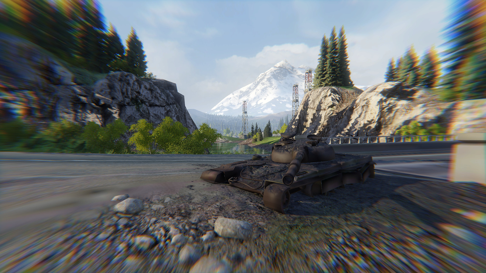
Armored Warfare: Project Armata is a free online tank action game developed by Allods Team, the game studio MY.GAMES. Despite the fact that the game is made on CryEngine, a fairly popular engine with a good realtime render, for our game we have to modify and create a lot from scratch. In this article, I want to talk about how we implemented chromatic aberration for the first person view, and what it is.
What is chromatic aberration?
Chromatic aberration is a lens defect in which not all colors arrive at the same point. This is due to the fact that the refractive index of the medium depends on the wavelength of light (see dispersion ). For example, this is how the situation looks when the lens does not suffer from chromatic aberration:
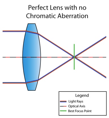
And here is a lens with a defect:
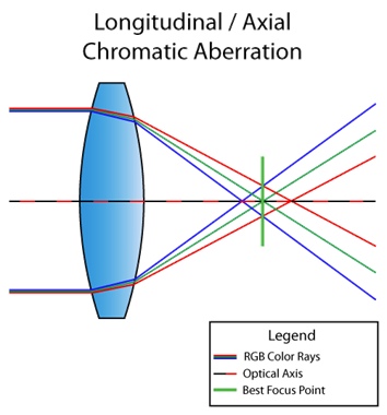
By the way, the situation above is called longitudinal (or axial) chromatic aberration. It occurs when different wavelengths do not converge at the same point in the focal plane after passing through the lens. Then the defect is visible in the whole picture:
In the picture above, you can see that purple and green colors stand out due to a defect. Can not see? And in this picture?

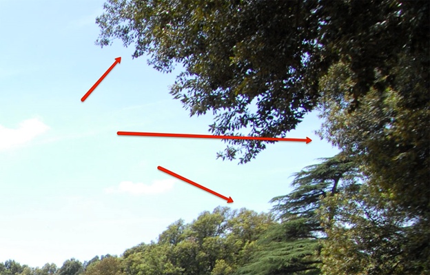
There is also lateral (or lateral) chromatic aberration. It occurs when light is incident at an angle to the lens. As a result, different wavelengths of light converge at different points in the focal plane. Here's a picture for you to understand:
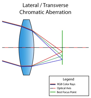
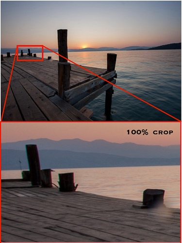
You can already see from the diagram that as a result we get a complete decomposition of light from red to violet. Unlike longitudinal, lateral chromatic aberration never appears in the center, only closer to the edges of the image. So that you understand what I mean, here's another picture from the Internet:
Well, since we're done with theory, let's get to the point.
Lateral chromatic aberration with light decomposition
I'll start with the fact that I will answer the question that could arise in the head of many of you: "Isn't CryEngine implemented chromatic aberration?" There is. But it is used at the post-processing stage in the same shader with sharpening, and the algorithm looks like this ( link to the code ):
screenColor.r = shScreenTex.SampleLevel( shPointClampSampler, (IN.baseTC.xy - 0.5) * (1 + 2 * psParams[0].x * CV_ScreenSize.zw) + 0.5, 0.0f).r;
screenColor.b = shScreenTex.SampleLevel( shPointClampSampler, (IN.baseTC.xy - 0.5) * (1 - 2 * psParams[0].x * CV_ScreenSize.zw) + 0.5, 0.0f).b;
Which, in principle, works. But we have a game about tanks. We need this effect only for the first person view, and only for beauty, that is, so that everything is in focus in the center (hello to lateral aberration). Therefore, the current implementation did not suit at least the fact that its effect was visible throughout the picture.
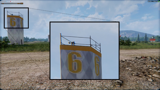
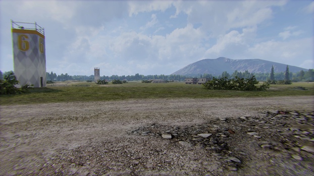
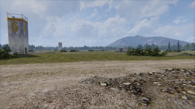
This is what the aberration itself looked like (attention to the left side):
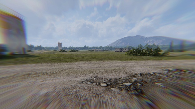
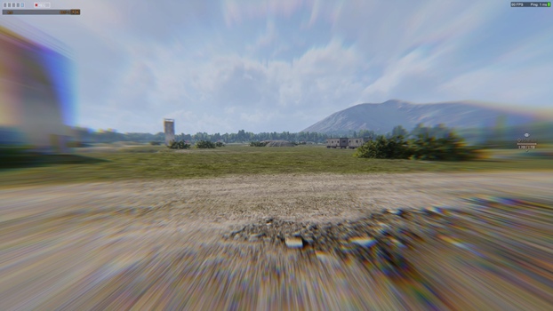
And this is how it looked if you twist the parameters:

Therefore, we have set as our goal:
- Implement lateral chromatic aberration so that everything is in focus near the scope, and if characteristic color defects are not visible on the sides, then at least to be blurred.
- Sample a texture by multiplying RGB channels by coefficients corresponding to a specific wavelength. I haven't talked about this yet, so now it may not be entirely clear what this point is about. But we will definitely consider it in all details later.
First, let's look at the general mechanism and code for creating lateral chromatic aberration.
half distanceStrength = pow(length(IN.baseTC - 0.5), falloff);
half2 direction = normalize(IN.baseTC.xy - 0.5);
half2 velocity = direction * blur * distanceStrength;
So, first, a circular mask is built, which is responsible for the distance from the center of the screen, then the direction from the center of the screen is calculated, and then all this is multiplied with
blur. Blurand falloff- these are parameters that are passed from the outside and are just multipliers for adjusting the aberration. Also, a parameter is thrown from the outside sampleCount, which is responsible not only for the number of samples, but also, in fact, for the step between the sampling points, since
half2 offsetDecrement = velocity * stepMultiplier / half(sampleCount);
Now we just have to go
sampleCountonce from a given point of the texture, shifting each time by offsetDecrement, multiply the channels by the corresponding wave weights and divide by the sum of these weights. Well, it's time to talk about the second point of our global goal.
The visible spectrum of light ranges from 380 nm (violet) to 780 nm (red). And lo and behold, the wavelength can be converted to RGB palette. In Python, the code that does this magic looks like this:
def get_color(waveLength):
    if waveLength >= 380 and waveLength < 440:
        red = -(waveLength - 440.0) / (440.0 - 380.0)
        green = 0.0
        blue  = 1.0
    elif waveLength >= 440 and waveLength < 490:
        red   = 0.0
        green = (waveLength - 440.0) / (490.0 - 440.0)
        blue  = 1.0
    elif waveLength >= 490 and waveLength < 510:
        red   = 0.0
        green = 1.0
        blue  = -(waveLength - 510.0) / (510.0 - 490.0)
    elif waveLength >= 510 and waveLength < 580:
        red   = (waveLength - 510.0) / (580.0 - 510.0)
        green = 1.0
        blue  = 0.0
    elif waveLength >= 580 and waveLength < 645:
        red   = 1.0
        green = -(waveLength - 645.0) / (645.0 - 580.0)
        blue  = 0.0
    elif waveLength >= 645 and waveLength < 781:
        red   = 1.0
        green = 0.0
        blue  = 0.0
    else:
        red   = 0.0
        green = 0.0
        blue  = 0.0

    factor = 0.0
    if waveLength >= 380 and waveLength < 420:
        factor = 0.3 + 0.7*(waveLength - 380.0) / (420.0 - 380.0)
    elif waveLength >= 420 and waveLength < 701:
        factor = 1.0
    elif waveLength >= 701 and waveLength < 781:
        factor = 0.3 + 0.7*(780.0 - waveLength) / (780.0 - 700.0)

    gamma = 0.80
    R = (red   * factor)**gamma if red > 0 else 0
    G = (green * factor)**gamma if green > 0 else 0
    B = (blue  * factor)**gamma if blue > 0 else 0

    return R, G, B
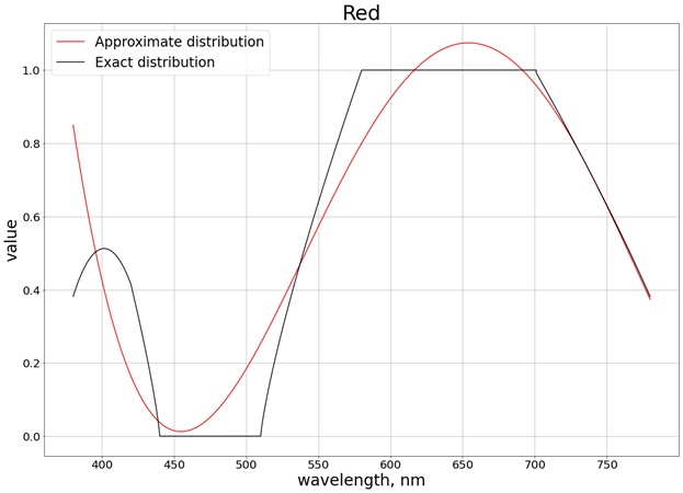
As a result, we get the following color distribution:

In short, the graph shows how much and what color is contained in a wave with a specific length. On the ordinate axis, we just get the same weights that I spoke about earlier. Now we can fully implement the algorithm, taking into account the previously stated:
half3 accumulator = (half3) 0;
half2 offset = (half2) 0;
half3 WeightSum = (half3) 0;
half3 Weight = (half3) 0;
half3 color;
half waveLength;

for (int i = 0; i < sampleCount; i++)
{
    waveLength = lerp(startWaveLength, endWaveLength, (half)(i) / (sampleCount - 1.0));
    Weight.r = GetRedWeight(waveLength);
    Weight.g = GetGreenWeight(waveLength);
    Weight.b = GetBlueWeight(waveLength);

    offset -= offsetDecrement;

    color = tex2Dlod(baseMap, half4(IN.baseTC + offset, 0, 0)).rgb;
    accumulator.rgb += color.rgb * Weight.rgb;

    WeightSum.rgb += Weight.rgb;
}

OUT.Color.rgb = half4(accumulator.rgb / WeightSum.rgb, 1.0);
That is, the idea is that the more we have
sampleCount, the less step we have between the sample points, and the more we disperse the light (we take into account more waves with different lengths).
If it is still not clear, then let's look at a specific example, namely our first attempt, and I will explain what to take for
startWaveLengthand endWaveLength, and how the functions will be implemented GetRed(Green, Blue)Weight.
Fitting the entire visible spectrum
So, from the graph above, we know the approximate ratio and approximate values of the RGB palette for each wavelength. For example, for a wavelength of 380 nm (violet) (see the same graph), we see that RGB (0.4, 0, 0.4). It is these values that we take for the weights that I spoke about earlier.
Now let's try to get rid of the function of obtaining color by a polynomial of the fourth degree, so that the calculations are cheaper (we are not a Pixar studio, but a game studio: the cheaper the calculations, the better). This fourth-degree polynomial should approximate the resulting graphs. To build the polynomial, I used the SciPy library:
wave_arange = numpy.arange(380, 780, 0.001)
red_func = numpy.polynomial.polynomial.Polynomial.fit(wave_arange, red, 4)
As a result, the following result is obtained (I have divided into 3 separate graphs corresponding to each separate channel, so that it is easier to compare with the exact value):
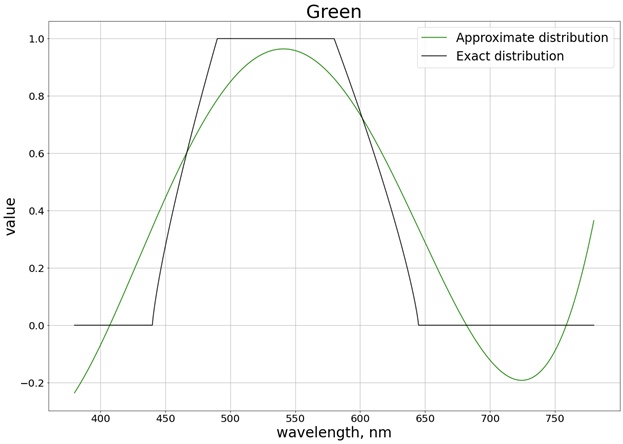
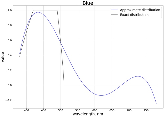
To ensure that the values do not go beyond the limit of the segment [0, 1], we use the function
saturate. For red, for example, the function is obtained:
half GetRedWeight(half x)
{
    return saturate(0.8004883122689207 +
    1.3673160565954385 * (-2.9000047500568042 + 0.005000012500149485 * x) -
    1.244631137356407 * pow(-2.9000047500568042 + 0.005000012500149485 * x, 2) - 1.6053230172845554 * pow(-2.9000047500568042 + 0.005000012500149485*x, 3)+ 1.055933936470091 * pow(-2.9000047500568042 + 0.005000012500149485*x, 4));
}
The missing parameters
startWaveLengthand endWaveLengthin this case are 780 nm and 380 nm, respectively. The result in practice sampleCount=3is the following (see the edges of the picture):
If we tweak the values, increase
sampleCountto 400, then everything becomes better:
Unfortunately, we have a realtime render in which we cannot allow 400 samples (about 3-4) in one shader. Therefore, we slightly reduced the wavelength range.
Part of the visible spectrum
Let's take a range so that we end up with both pure red and pure blue colors. We also refuse the red tail on the left, as it greatly affects the final polynomial. As a result, we get the distribution on the segment [440, 670]:

Also, there is no need to interpolate over the entire segment, since now we can get a polynomial only for the segment where the value changes. For example, for the red color, this is the segment [510, 580], where the weight value varies from 0 to 1. In this case, you can get a second-order polynomial, which is then
saturatealso reduced by the function to the range of values [0, 1]. For all three colors we get the following result with saturation taken into account:

As a result, we get, for example, the following polynomial for red:
half GetRedWeight(half x)
{
    return saturate(0.5764348105166407 +
    0.4761860550080825 * (-15.571636738012254 + 0.0285718367412005 * x) -
    0.06265740390367036 * pow(-15.571636738012254 + 0.0285718367412005 * x, 2));
}
And in practice with
sampleCount=3:
In this case, with the twisted settings, approximately the same result is obtained as when sampling over the entire range of the visible spectrum:
Thus, with polynomials of the second degree, we got a good result in the wavelength range from 440 nm to 670 nm.
Optimization
In addition to optimizing the calculations with polynomials, you can optimize the shader's work, relying on the mechanism that we laid in the basis of our lateral chromatic aberration, namely, do not carry out calculations in the area where the total displacement does not go beyond the current pixel, otherwise we will sample the same pixel, and we get it.
It looks like this:
bool isNotAberrated = abs(offsetDecrement.x * g_VS_ScreenSize.x) < 1.0 && abs(offsetDecrement.y * g_VS_ScreenSize.y) < 1.0;
if (isNotAberrated)
{
    OUT.Color.rgb = tex2Dlod(baseMap, half4(IN.baseTC, 0, 0)).rgb;
    return OUT;
}
The optimization is small, but very proud.
Conclusion
The lateral chromatic aberration itself looks very cool; this defect does not interfere with the sight in the center. The idea of decomposing light into weights is a very interesting experiment that can give a completely different picture if your engine or game allows more than three samples. In our case, it was possible not to bother and come up with a different algorithm, since even with optimizations we cannot afford many samples, and, for example, the difference between 3 and 5 samples is not very visible. You can experiment with the described method yourself and see the results.