where q is the charge of the particle, r ij is the distance between particles, C is some constant depending on the choice of units of measurement. In SI it is -, in SGS - 1, in my program (where energy is expressed in electron volts, distance in angstroms, and charge in elementary charges) C is approximately equal to 14.3996.
So what, you say? Just add the corresponding term to the pair potential and you're done. However, most often in MD modeling, periodic boundary conditions are used, i.e. the simulated system is surrounded from all sides by an infinite number of its virtual copies. In this case, each virtual image of our system will interact with all charged particles inside the system according to Coulomb's law. And since the Coulomb interaction decreases very weakly with distance (like 1 / r), then it is not so easy to dismiss it, saying that we cannot calculate it from such and such a distance. A series of the form 1 / x diverges, i.e. its amount, in principle, can grow indefinitely. And now, don't you salt a bowl of soup? Will it kill you with electricity?
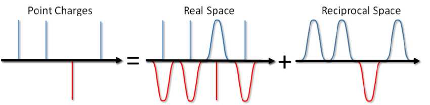
... you can not only salt the soup, but also calculate the energy of the Coulomb interaction under periodic boundary conditions. This method was proposed by Ewald back in 1921 for calculating the energy of an ionic crystal (you can also see it on Wikipedia ). The essence of the method is to screen point charges and then subtract the screening function. In this case, a part of the electrostatic interaction is reduced to a short-acting one and it can be simply cut off in a standard way. The remaining long-range part is effectively summed in Fourier space. Omitting the conclusion, which can be viewed in Blinov's article or in the same book by Frenkel and Smith , I will immediately write down a solution called the Ewald sum:
where α is a parameter that regulates the ratio of calculations in forward and reverse spaces, k are vectors in reciprocal space over which summation is taking place, V is the volume of the system (in forward space). The first part (E real ) is short-range and is calculated in the same cycle as the other pair potentials, see the real_ewald function in the previous article. The last contribution (E onst ) is a correction for self-interaction and is often called the "constant part" because it does not depend on the coordinates of the particles. Its calculation is trivial, so we will focus only on the second part of the Ewald sum (E rec), summation in reciprocal space. Naturally, at the time of Ewald's derivation, there was no molecular dynamics; I could not find who first used this method in MD. Nowadays, any book on MD contains its presentation as a kind of gold standard. To book, Allen even supplied example code in Fortran. Fortunately, I still have the code that was once written in C for the sequential version, I just need to parallelize it (I allowed myself to omit some variable declarations and other unimportant details):
void ewald_rec()
{
    int mmin = 0;
    int nmin = 1;

    //    iexp(x[i] * kx[l]),
    double** elc;
    double** els;
    //... iexp(y[i] * ky[m])
    double** emc;
    double** ems;
    //... iexp(z[i] * kz[n]),
    double** enc;
    double** ens;

    //     iexp(x*kx)*iexp(y*ky)
    double* lmc;
    double* lms;
    //   q[i] * iexp(x*kx)*iexp(y*ky)*iexp(z*kz)
    double* ckc;
    double* cks;

    //
    eng = 0.0;
    for (i = 0; i < Nat; i++)   //
    {
        // emc/s[i][0]  enc/s[i][0]
        //   elc/s  , .
        elc[i][0] = 1.0;
        els[i][0] = 0.0;

        // iexp(kr)
        sincos(twopi * xs[i] * ra, els[i][1], elc[i][1]);
        sincos(twopi * ys[i] * rb, ems[i][1], emc[i][1]);
        sincos(twopi * zs[i] * rc, ens[i][1], enc[i][1]);
    }

    //     emc/s[i][l] = iexp(y[i]*ky[l]) ,
    for (l = 2; l < ky; l++)
        for (i = 0; i < Nat; i++)
        {
            emc[i][l] = emc[i][l - 1] * emc[i][1] - ems[i][l - 1] * ems[i][1];
            ems[i][l] = ems[i][l - 1] * emc[i][1] + emc[i][l - 1] * ems[i][1];
        }

    //     enc/s[i][l] = iexp(z[i]*kz[l]) ,
    for (l = 2; l < kz; l++)
        for (i = 0; i < Nat; i++)
        {
            enc[i][l] = enc[i][l - 1] * enc[i][1] - ens[i][l - 1] * ens[i][1];
            ens[i][l] = ens[i][l - 1] * enc[i][1] + enc[i][l - 1] * ens[i][1];
        }

    //     K-:
    for (l = 0; l < kx; l++)
    {
        rkx = l * twopi * ra;
        //  exp(ikx[l])  ikx[0]
        if (l == 1)
            for (i = 0; i < Nat; i++)
            {
                elc[i][0] = elc[i][1];
                els[i][0] = els[i][1];
            }
        else if (l > 1)
            for (i = 0; i < Nat; i++)
            {
                // iexp(kx[0]) = iexp(kx[0]) * iexp(kx[1])
                x = elc[i][0];
                elc[i][0] = x * elc[i][1] - els[i][0] * els[i][1];
                els[i][0] = els[i][0] * elc[i][1] + x * els[i][1];
            }

        for (m = mmin; m < ky; m++)
        {
            rky = m * twopi * rb;
            //     iexp(kx*x[i]) * iexp(ky*y[i])
            if (m >= 0)
                for (i = 0; i < Nat; i++)
                {
                    lmc[i] = elc[i][0] * emc[i][m] - els[i][0] * ems[i][m];
                    lms[i] = els[i][0] * emc[i][m] + ems[i][m] * elc[i][0];
                }
            else //    m   :
                for (i = 0; i < Nat; i++)
                {
                    lmc[i] = elc[i][0] * emc[i][-m] + els[i][0] * ems[i][-m];
                    lms[i] = els[i][0] * emc[i][-m] - ems[i][-m] * elc[i][0];
                }

            for (n = nmin; n < kz; n++)
            {
                rkz = n * twopi * rc;
                rk2 = rkx * rkx + rky * rky + rkz * rkz;
                if (rk2 < rkcut2) //
                {
                    //   (q[i]*iexp(kr[k]*r[i])) -
                    sumC = 0; sumS = 0;
                    if (n >= 0)
                        for (i = 0; i < Nat; i++)
                        {
                            //
                            ch = charges[types[i]].charge;

                            ckc[i] = ch * (lmc[i] * enc[i][n] - lms[i] * ens[i][n]);
                            cks[i] = ch * (lms[i] * enc[i][n] + lmc[i] * ens[i][n]);

                            sumC += ckc[i];
                            sumS += cks[i];
                        }
                    else //      :
                        for (i = 0; i < Nat; i++)
                        {
                            //
                            ch = charges[types[i]].charge;

                            ckc[i] = ch * (lmc[i] * enc[i][-n] + lms[i] * ens[i][-n]);
                            cks[i] = ch * (lms[i] * enc[i][-n] - lmc[i] * ens[i][-n]);

                            sumC += ckc[i];
                            sumS += cks[i];
                        }

                    //
                    akk = exp(rk2 * elec->mr4a2) / rk2;
                    eng += akk * (sumC * sumC + sumS * sumS);

                    for (i = 0; i < Nat; i++)
                    {
                        x = akk * (cks[i] * sumC - ckc[i] * sumS) * C * twopi * 2 * rvol;
                        fxs[i] += rkx * x;
                        fys[i] += rky * x;
                        fzs[i] += rkz * x;
                    }

                }
            } // end n-loop (over kz-vectors)

            nmin = 1 - kz;

        } // end m-loop (over ky-vectors)

        mmin = 1 - ky;

    }  // end l-loop (over kx-vectors)


   engElec2 = eng *  * twopi * rvol;
}
A couple of explanations for the code: the function calculates the complex exponent (in the comments to the code it is denoted iexp to remove the imaginary unit from the brackets) from the vector product of the k-vector and the radius vector of the particle for all k-vectors and for all particles. This exponent is multiplied by the particle charge. Next, the sum of such products for all particles is calculated (the internal sum in the formula for E rec ), in Frenkel it is called the charge density, and in Blinov it is called the structural factor. And then, on the basis of these structural factors, the energy and forces acting on the particles are calculated. The components of k-vectors (2π * l / a, 2π * m / b, 2π * n / c) are characterized by three integers l , m and n, which run in cycles up to user-specified limits. Parameters a, b and c are the dimensions of the simulated system in dimensions x, y and z, respectively (the conclusion is correct for a system with a rectangular parallelepiped geometry). In the code, 1 / a , 1 / b, and 1 / c correspond to the variables ra , rb, and rc . Arrays for each value are presented in two copies: for the real and imaginary parts. Each next k-vector in one dimension is obtained iteratively from the previous one by complex multiplying the previous one by one, so as not to count the sine with cosine each time. The emc / s and enc / s arrays are populated for all mand n , respectively, and the array elc / s places the value for each l > 1 in the zero index of l in order to save memory.
For the purpose of parallelization, it is advantageous to "reverse" the order of the cycles so that the outer cycle runs over the particles. And here we see a problem - this function can be parallelized only before calculating the sum over all particles (charge density). Further calculations are based on this amount, and it will be calculated only when all threads finish their work, so you have to split this function into two. The first calculates the charge density, and the second calculates the energy and forces. Note that the second function will again require the quantity q iiexp (kr) for each particle and for each k-vector, calculated in the previous step. And here there are two approaches: either recalculate it again, or remember it.
The first option takes more time, the second - more memory (number of particles * number of k-vectors * sizeof (float2)). I settled on the second option:
__global__ void recip_ewald(int atPerBlock, int atPerThread, cudaMD* md)
// calculate reciprocal part of Ewald summ
// the first part : summ (qiexp(kr)) evaluation
{
    int i;      // for atom loop
    int ik;     // index of k-vector
    int l, m, n;
    int mmin = 0;
    int nmin = 1;
    float tmp, ch;
    float rkx, rky, rkz, rk2;   // component of rk-vectors

    int nkx = md->nk.x;
    int nky = md->nk.y;
    int nkz = md->nk.z;

    // arrays for keeping iexp(k*r) Re and Im part
    float2 el[2];
    float2 em[NKVEC_MX];
    float2 en[NKVEC_MX];

    float2 sums[NTOTKVEC];          // summ (q iexp (k*r)) for each k
    extern __shared__ float2 sh_sums[];     // the same in shared memory

    float2 lm;     // temp var for keeping el*em
    float2 ck;     // temp var for keeping q * el * em * en (q iexp (kr))

    // invert length of box cell
    float ra = md->revLeng.x;
    float rb = md->revLeng.y;
    float rc = md->revLeng.z;

    if (threadIdx.x == 0)
        for (i = 0; i < md->nKvec; i++)
            sh_sums[i] = make_float2(0.0f, 0.0f);
    __syncthreads();

    for (i = 0; i < md->nKvec; i++)
        sums[i] = make_float2(0.0f, 0.0f);

    int id0 = blockIdx.x * atPerBlock + threadIdx.x * atPerThread;
    int N = min(id0 + atPerThread, md->nAt);

    ik = 0;
    for (i = id0; i < N; i++)
    {
        // save charge
        ch = md->specs[md->types[i]].charge;

        el[0] = make_float2(1.0f, 0.0f);    // .x - real part (or cos) .y - imagine part (or sin)

        em[0] = make_float2(1.0f, 0.0f);
        en[0] = make_float2(1.0f, 0.0f);

        // iexp (ikr)
        sincos(d_2pi * md->xyz[i].x * ra, &(el[1].y), &(el[1].x));
        sincos(d_2pi * md->xyz[i].y * rb, &(em[1].y), &(em[1].x));
        sincos(d_2pi * md->xyz[i].z * rc, &(en[1].y), &(en[1].x));

        // fil exp(iky) array by complex multiplication
        for (l = 2; l < nky; l++)
        {
             em[l].x = em[l - 1].x * em[1].x - em[l - 1].y * em[1].y;
             em[l].y = em[l - 1].y * em[1].x + em[l - 1].x * em[1].y;
        }

        // fil exp(ikz) array by complex multiplication
        for (l = 2; l < nkz; l++)
        {
             en[l].x = en[l - 1].x * en[1].x - en[l - 1].y * en[1].y;
             en[l].y = en[l - 1].y * en[1].x + en[l - 1].x * en[1].y;
        }

        // MAIN LOOP OVER K-VECTORS:
        for (l = 0; l < nkx; l++)
        {
            rkx = l * d_2pi * ra;

            // move exp(ikx[l]) to ikx[0] for memory saving (ikx[i>1] are not used)
            if (l == 1)
                el[0] = el[1];
            else if (l > 1)
                {
                    // exp(ikx[0]) = exp(ikx[0]) * exp(ikx[1])
                    tmp = el[0].x;
                    el[0].x = tmp * el[1].x - el[0].y * el[1].y;
                    el[0].y = el[0].y * el[1].x + tmp * el[1].y;
                }

            //ky - loop:
            for (m = mmin; m < nky; m++)
            {
                rky = m * d_2pi * rb;

                //set temporary variable lm = e^ikx * e^iky
                if (m >= 0)
                {
                        lm.x = el[0].x * em[m].x - el[0].y * em[m].y;
                        lm.y = el[0].y * em[m].x + em[m].y * el[0].x;
                }
                else // for negative ky give complex adjustment to positive ky:
                {
                        lm.x = el[0].x * em[-m].x + el[0].y * em[-m].y;
                        lm.y = el[0].y * em[-m].x - em[-m].x * el[0].x;
                }

                //kz - loop:
                for (n = nmin; n < nkz; n++)
                {
                    rkz = n * d_2pi * rc;
                    rk2 = rkx * rkx + rky * rky + rkz * rkz;
                    if (rk2 < md->rKcut2) // cutoff
                    {
                        // calculate summ[q iexp(kr)]   (local part)
                        if (n >= 0)
                         {
                                ck.x = ch * (lm.x * en[n].x - lm.y * en[n].y);
                                ck.y = ch * (lm.y * en[n].x + lm.x * en[n].y);
                         }
                        else // for negative kz give complex adjustment to positive kz:
                         {
                                ck.x = ch * (lm.x * en[-n].x + lm.y * en[-n].y);
                                ck.y = ch * (lm.y * en[-n].x - lm.x * en[-n].y);
                        }
                        sums[ik].x += ck.x;
                        sums[ik].y += ck.y;

                        // save qiexp(kr) for each k for each atom:
                        md->qiexp[i][ik] = ck;
                        ik++;
                    }
                } // end n-loop (over kz-vectors)

                nmin = 1 - nkz;

            } // end m-loop (over ky-vectors)
            mmin = 1 - nky;
        }  // end l-loop (over kx-vectors)
    } // end loop by atoms

    // save sum into shared memory
    for (i = 0; i < md->nKvec; i++)
    {
        atomicAdd(&(sh_sums[i].x), sums[i].x);
        atomicAdd(&(sh_sums[i].y), sums[i].y);
    }
    __syncthreads();

    //...and to global
    int step = ceil((double)md->nKvec / (double)blockDim.x);
    id0 = threadIdx.x * step;
    N = min(id0 + step, md->nKvec);
    for (i = id0; i < N; i++)
    {
        atomicAdd(&(md->qDens[i].x), sh_sums[i].x);
        atomicAdd(&(md->qDens[i].y), sh_sums[i].y);
    }
}
// end 'ewald_rec' function

__global__ void ewald_force(int atPerBlock, int atPerThread, cudaMD* md)
// calculate reciprocal part of Ewald summ
// the second part : enegy and forces
{
    int i;      // for atom loop
    int ik;     // index of k-vector
    float tmp;

    // accumulator for force components
    float3 force;

    // constant factors for energy and force
    float eScale = md->ewEscale;
    float fScale = md->ewFscale;

    int id0 = blockIdx.x * atPerBlock + threadIdx.x * atPerThread;
    int N = min(id0 + atPerThread, md->nAt);
    for (i = id0; i < N; i++)
    {
        force = make_float3(0.0f, 0.0f, 0.0f);

        // summ by k-vectors
        for (ik = 0; ik < md->nKvec; ik++)
        {
            tmp = fScale * md->exprk2[ik] * (md->qiexp[i][ik].y * md->qDens[ik].x - md->qiexp[i][ik].x * md->qDens[ik].y);

            force.x += tmp * md->rk[ik].x;
            force.y += tmp * md->rk[ik].y;
            force.z += tmp * md->rk[ik].z;
        }

        md->frs[i].x += force.x;
        md->frs[i].y += force.y;
        md->frs[i].z += force.z;
    } // end loop by atoms


    // one block calculate energy
    if (blockIdx.x == 0)
        if (threadIdx.x == 0)
        {
            for (ik = 0; ik < md->nKvec; ik++)
                md->engCoul2 += eScale * md->exprk2[ik] * (md->qDens[ik].x * md->qDens[ik].x + md->qDens[ik].y * md->qDens[ik].y);
        }

}
// end 'ewald_force' function
I hope you will forgive me for leaving comments in English, the code is practically the same as the serial version. The code even became more readable due to the fact that arrays lost one dimension: elc / s [i] [l] , emc / s [i] [m] and enc / s [i] [n] turned into one-dimensional el , em and en , arrays lmc / s and ckc / s - into the variables lm and ck (dimension by particles has disappeared, since there is no longer the need to store it for each particle, the intermediate result is accumulated in shared memory). Unfortunately, a problem immediately arose: the arrays em and enhad to be set static so as not to use global memory and not dynamically allocate memory each time. The number of elements in them is determined by the NKVEC_MX directive (the maximum number of k-vectors in one dimension) at the compilation stage, and only the first nky / z elements are used at runtime. In addition, an end-to-end index on all k-vectors and a similar directive appeared, limiting the total number of these vectors NTOTKVEC . The problem will arise if the user needs more k-vectors than specified by the directives. To calculate the energy, a block with a zero index is provided, since it does not matter which block will perform this calculation and in what order. Note that the value calculated in the variable akkthe serial code depends only on the size of the simulated system and can be calculated at the initialization stage, in my implementation it is stored in the md-> exprk2 [] array for each k-vector. Similarly, the components of k-vectors are taken from the md-> rk [] array . Here it might be necessary to use ready-made FFT functions, since the method is based on it, but I still did not figure out how to do it.
Well, now let's try to count something, but the same sodium chloride. Let's take 2 thousand sodium ions and the same amount of chlorine. Let us set the charges as integers, and take pair potentials, for example, from this work. Let's set the starting configuration randomly and mix it slightly, Figure 2a. We choose the volume of the system so that it corresponds to the density of sodium chloride at room temperature (2.165 g / cm 3 ). Let's start all this for a short time (10'000 steps of 5 femtoseconds) with naive consideration of electrostatics according to Coulomb's law and using Ewald summation. The resulting configurations are shown in Figures 2b and 2c, respectively. It seems that in the case of Ewald, the system is a little more streamlined than without him. It is also important that the total energy fluctuations have significantly decreased with the use of summation.
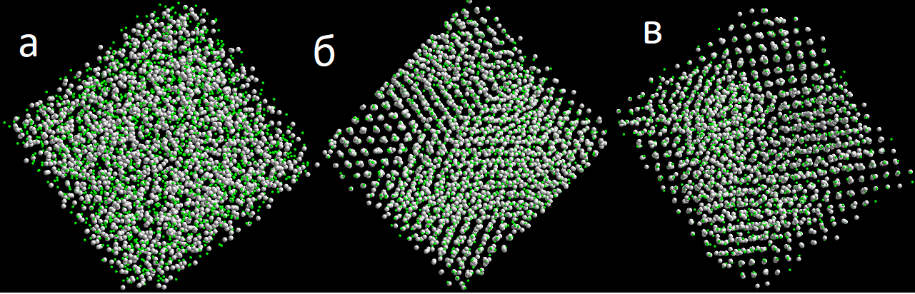
Figure 2. Initial configuration of the NaCl system (a) and after 10'000 integration steps: naive method (b) and with the Ewald scheme (c).
Instead of a conclusion
Note that the structure obtained in the figure does not correspond to the NaCl crystal lattice, but rather to the ZnS lattice, but this is already a complaint about pair potentials. Taking into account electrostatics is very important for molecular dynamics modeling. It is believed that it is the electrostatic interaction that is responsible for the formation of crystal lattices, since it acts at large distances. True, from this position it is difficult to explain how substances such as argon crystallize during cooling.
In addition to the Ewald method mentioned, there are also other methods of accounting for electrostatics, see, for example, this review .