Once, on the eve of the client conference, which is held annually by the DAN group, we were thinking about what interesting things we can think of so that our partners and clients will have pleasant impressions and memories of the event. We decided to make out an archive of thousands of photos from this conference and several past (and there were 18 in all by that time): a person sends us his photo, and in a couple of seconds we send him a selection of photos with him for several years from our archives.
We did not invent a bicycle, we took the well-known dlib library and received embeddings (vector representations) of each person.
We added a Telegram bot for convenience, and everything was great. From the point of view of face recognition algorithms, everything worked with a bang, but the conference was over, and I did not want to part with the tried and tested technologies. From several thousand people I wanted to go to hundreds of millions, but we did not have a specific business task. After a while, our colleagues had a task that required working with such large amounts of data.
The question was to write a smart bot monitoring system inside the Instagram network. Here our thought gave rise to a simple and complex approach:
Simple way: We consider all accounts that have much more subscriptions than subscribers, no avatar, full name is not filled, etc. As a result, we get an incomprehensible crowd of half-dead accounts.
The hard way: Since modern bots have become much smarter, and now they post posts, sleep, and even write content, the question arises: how to catch these? First, keep a close eye on their friends, as they are often bots too, and keep track of duplicate photos. Secondly, rarely does a bot know how to generate its own photos (although this is possible), which means that duplicate photos of people in different accounts on Instagram are a good trigger for finding a network of bots.
What's next?
If the simple way is quite predictable and quickly yields some results, the difficult way is complicated precisely because for its implementation we will have to vectorize and index the similarities of incredibly large volumes of photographs - millions, even billions, for subsequent comparisons. How to put it into practice? After all, technical issues arise:
- Search speed and accuracy
- Disk space occupied by the data
- The size of RAM used.
If there were only a few photos, at least no more than ten thousand, we could limit ourselves to simple solutions with vector clustering, but to work with huge volumes of vectors and find the nearest neighbors to a certain vector, complex and optimized algorithms are required.
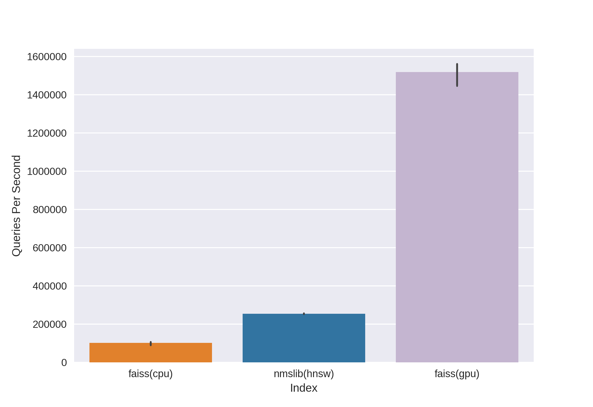
There are well-known and proven technologies such as Annoy, FAISS, HNSW. The fast HNSW neighbor search algorithm available in the nmslib and hnswlib libraries, shows state-of-the-art results on the CPU, which can be seen from the same benchmarks. But we cut it off right away, since we are not happy with the amount of memory used when working with really large amounts of data. We began to choose between Annoy and FAISS and ended up choosing FAISS because of convenience, less memory usage, potential use on GPUs and performance benchmarks (you can see, for example, here ). By the way, in FAISS, the HNSW algorithm is implemented as an option.
What is FAISS?
Facebook AI Research Similarity Search is a development of the Facebook AI Research team for quickly finding nearby neighbors and clustering in vector space. High search speed allows working with very large data - up to several billion vectors.
The main advantage of FAISS is its state-of-the-art results on the GPU, while its implementation on the CPU is slightly inferior to hnsw (nmslib). We wanted to be able to search on both the CPU and GPU. In addition, FAISS is optimized in terms of memory usage and search on large batches.
Source
FAISS allows you to quickly find the k nearest vectors for a given vector x. But how does this search work under the hood?
Indexes
The main concept in FAISS is index , and in essence it is just a collection of parameters and vectors. The parameter sets are completely different and depend on the user's needs. Vectors can remain unchanged, but can be rebuilt. Some indexes are available for work immediately after adding vectors to them, and some require prior training. Vector names are stored in the index: either in numbering from 0 to n, or as a number that fits into the Int64 type.
The first index, and the simplest one that we used at the conference, is Flat . It only stores all the vectors in itself, and the search for a given vector is performed by exhaustive search, so there is no need to train it (but more on training below). With a small amount of data, such a simple index can fully cover the needs of the search.
Example:
import numpy as np
dim = 512  #     512
nb = 10000  #
nq = 5 #
np.random.seed(228)
vectors = np.random.random((nb, dim)).astype('float32')
query = np.random.random((nq, dim)).astype('float32')
Create a Flat Index and add vectors without training:
import faiss
index = faiss.IndexFlatL2(dim)
print(index.ntotal)  #
index.add(vectors)
print(index.ntotal)  #    10 000
Now we find 7 nearest neighbors for the first five vectors from vectors:
topn = 7
D, I = index.search(vectors[:5], topn)  #  : Distances, Indices
print(I)
print(D)
Output
[[0 5662 6778 7738 6931 7809 7184]
 [1 5831 8039 2150 5426 4569 6325]
 [2 7348 2476 2048 5091 6322 3617]
 [3  791 3173 6323 8374 7273 5842]
 [4 6236 7548  746 6144 3906 5455]]

[[ 0.  71.53578  72.18823  72.74326  73.2243   73.333244 73.73317 ]
 [ 0.  67.604805 68.494774 68.84221  71.839905 72.084335 72.10817 ]
 [ 0.  66.717865 67.72709  69.63666  70.35903  70.933304 71.03237 ]
 [ 0.  68.26415  68.320595 68.82381  68.86328  69.12087  69.55179 ]
 [ 0.  72.03398  72.32417  73.00308  73.13054  73.76181  73.81281 ]]
We see that the closest neighbors with a distance of 0 are the vectors themselves, the rest are ranged by increasing distance. Let's search for our vectors from query:
D, I = index.search(query, topn)
print(I)
print(D)
Output
[[2467 2479 7260 6199 8640 2676 1767]
 [2623 8313 1500 7840 5031   52 6455]
 [1756 2405 1251 4136  812 6536  307]
 [3409 2930  539 8354 9573 6901 5692]
 [8032 4271 7761 6305 8929 4137 6480]]

[[73.14189  73.654526 73.89804  74.05615  74.11058  74.13567  74.443436]
 [71.830215 72.33813  72.973885 73.08897  73.27939  73.56996  73.72397 ]
 [67.49588  69.95635  70.88528  71.08078  71.715965 71.76285  72.1091  ]
 [69.11357  69.30089  70.83269  71.05977  71.3577   71.62457  71.72549 ]
 [69.46417  69.66577  70.47629  70.54611  70.57645  70.95326  71.032005]]
Now the distances in the first column of the results are not zero, since the vectors from query are not in the index.
The index can be saved to disk and then loaded from disk:
faiss.write_index(index, "flat.index")
index = faiss.read_index("flat.index")
It would seem that everything is elementary! A few lines of code - and we already got a structure for searching high-dimensional vectors. But such an index with only tens of millions of vectors of dimension 512 will weigh about 20GB and take up as much RAM when used.
In the project for the conference, we used just such a basic approach with a flat index, everything was great due to the relatively small amount of data, but now we are talking about tens and hundreds of millions of high-dimensional vectors!
Speed up searches with Inverted lists

Source
The main and coolest feature of FAISS is the IVF index, or Inverted File index. The idea of Inverted files is laconic, and beautifully explained on the fingers :
Let's imagine a gigantic army, consisting of the most motley warriors, numbering, say, 1,000,000 people. Commanding an entire army at once will be impossible. As is customary in military affairs, it is necessary to divide our army into units. Let's divide intoapproximately equal parts, choosing for the role of commanders a representative from each unit. And we will try to send as similar as possible in character, origin, physical data, etc. warriors in one unit, and we will choose the commander so that he represents his unit as accurately as possible - he is someone "average". As a result, our task was reduced from the command of a million soldiers to the command of the 1000th units through their commanders, and we have an excellent idea of the composition of our army, since we know what commanders are.
This is the idea behind the IVF index: let's group a large set of vectors piece by piece using the k-means algorithm, putting in correspondence to each part a centroid, is a vector that is the chosen center for a given cluster. We will search through the minimum distance to the centroid, and only then look for the minimum distances among the vectors in the cluster that corresponds to this centroid. Taking k equalwhere - the number of vectors in the index, we get the optimal search at two levels - first among centroid then among vectors in each cluster. Search is much faster than brute force search, which solves one of our problems when working with many millions of vectors.

The vector space is divided by the k-means method into k clusters. Each cluster is assigned a centroid.
Example code:
dim = 512
k = 1000  #  “”
quantiser = faiss.IndexFlatL2(dim)
index = faiss.IndexIVFFlat(quantiser, dim, k)
vectors = np.random.random((1000000, dim)).astype('float32')  # 1 000 000 “”
And you can write it much more elegantly, using the convenient FAISS thing to build the index:
index = faiss.index_factory(dim, “IVF1000,Flat”)
 :
print(index.is_trained)   # False.
index.train(vectors)  # Train

#  ,      ,      :
print(index.is_trained)  # True
print(index.ntotal)   # 0
index.add(vectors)
print(index.ntotal)   # 1000000
Having examined this type of index after Flat, we solved one of our potential problems - the search speed, which becomes several times lower compared to exhaustive search.
D, I = index.search(query, topn)
print(I)
print(D)
Output
[[19898 533106 641838 681301 602835 439794 331951]
 [654803 472683 538572 126357 288292 835974 308846]
 [588393 979151 708282 829598  50812 721369 944102]
 [796762 121483 432837 679921 691038 169755 701540]
 [980500 435793 906182 893115 439104 298988 676091]]

[[69.88127  71.64444  72.4655   72.54283  72.66737  72.71834  72.83057]
 [72.17552  72.28832  72.315926 72.43405  72.53974  72.664055 72.69495]
 [67.262115 69.46998  70.08826  70.41119  70.57278  70.62283  71.42067]
 [71.293045 71.6647   71.686615 71.915405 72.219505 72.28943  72.29849]
 [73.27072  73.96091  74.034706 74.062515 74.24464  74.51218  74.609695]]
But there is one "but" - the search accuracy, as well as the speed, will depend on the number of visited clusters, which can be set using the nprobe parameter:
print(index.nprobe)  # 1 –
index.nprobe = 16  #   -16    top-n
D, I = index.search(query, topn)
print(I)
print(D)
Output
[[ 28707 811973  12310 391153 574413  19898 552495]
 [540075 339549 884060 117178 878374 605968 201291]
 [588393 235712 123724 104489 277182 656948 662450]
 [983754 604268  54894 625338 199198  70698  73403]
 [862753 523459 766586 379550 324411 654206 871241]]

[[67.365585 67.38003  68.17187  68.4904   68.63618  69.88127  70.3822]
 [65.63759  67.67015  68.18429  68.45782  68.68973  68.82755  69.05]
 [67.262115 68.735535 68.83473  68.88733  68.95465  69.11365  69.33717]
 [67.32007  68.544685 68.60204  68.60275  68.68633  68.933334 69.17106]
 [70.573326 70.730286 70.78615  70.85502  71.467674 71.59512  71.909836]]
As you can see, after increasing nprobe, we have completely different results, the top of the smallest distances in D got better.
You can take nprobe equal to the number of centroids in the index, then it will be equivalent to a brute force search, the accuracy will be the highest, but the search speed will noticeably decrease.
Searching the disk - On Disk Inverted Lists
Great, we solved the first problem, now we get an acceptable search speed on tens of millions of vectors! But all this is useless as long as our huge index does not fit into RAM.
Specifically for our task, the main advantage of FAISS is the ability to store Inverted Lists IVF indexes on disk, loading only metadata into RAM.
How do we create such an index: we train indexIVF with the necessary parameters on the maximum possible amount of data that fits into memory, then add vectors (those who have been trained and not only) to the trained index in parts and write the index for each of the parts to disk.
index = faiss.index_factory(512, “,IVF65536, Flat”, faiss.METRIC_L2)We train the index on the GPU in this way:
res = faiss.StandardGpuResources()
index_ivf = faiss.extract_index_ivf(index)
index_flat = faiss.IndexFlatL2(512)
clustering_index = faiss.index_cpu_to_gpu(res, 0, index_flat)  #  0 –  GPU
index_ivf.clustering_index = clustering_index
faiss.index_cpu_to_gpu (res, 0, index_flat) can be replaced with faiss.index_cpu_to_all_gpus (index_flat) to use all GPUs together.
It is highly desirable that the training sample is as representative as possible and has a uniform distribution, so we compose the training dataset in advance from the required number of vectors, randomly selecting them from the entire dataset.
train_vectors = ...  #
index.train(train_vectors)

#    ,   :
faiss.write_index(index, "trained_block.index")

#
#      :
for bno in range(first_block, last_block+ 1):
    block_vectors = vectors_parts[bno]
    block_vectors_ids = vectors_parts_ids[bno]  # id ,
    index = faiss.read_index("trained_block.index")
    index.add_with_ids(block_vectors, block_vectors_ids)
    faiss.write_index(index, "block_{}.index".format(bno))
After that, we combine all the Inverted Lists together. This is possible, since each of the blocks is essentially the same trained index, just with different vectors inside.
ivfs = []
for bno in range(first_block, last_block+ 1):
    index = faiss.read_index("block_{}.index".format(bno), faiss.IO_FLAG_MMAP)
    ivfs.append(index.invlists)
    #  index   inv_lists
    #        :
    index.own_invlists = False

#   :
index = faiss.read_index("trained_block.index")

#   invlists
#  invlists       merged_index.ivfdata
invlists = faiss.OnDiskInvertedLists(index.nlist, index.code_size, "merged_index.ivfdata")
ivf_vector = faiss.InvertedListsPtrVector()

for ivf in ivfs:
    ivf_vector.push_back(ivf)

ntotal = invlists.merge_from(ivf_vector.data(), ivf_vector.size())
index.ntotal = ntotal  #
index.replace_invlists(invlists)
faiss.write_index(index, data_path + "populated.index")  #
Bottom line: now our index is populated.index and merged_blocks.ivfdata files .
The populated.index contains the original full path to the file with Inverted Lists, so if the path to the ivfdata file changes for some reason, when reading the index, you will need to use the faiss.IO_FLAG_ONDISK_SAME_DIR flag , which allows you to search for the ivfdata file in the same directory as populated.index:
index = faiss.read_index('populated.index', faiss.IO_FLAG_ONDISK_SAME_DIR)
The demo example from the Github FAISS project was taken as the basis .
A mini-guide for choosing an index can be found in the FAISS Wiki . For example, we were able to put a training dataset of 12 million vectors in RAM, so we chose the IVFFlat index on 262144 centroids, and then scaled to hundreds of millions. It is also proposed to use the index IVF262144_HNSW32 in the guide, in which the affiliation of a vector to a cluster is determined by the HNSW algorithm with 32 nearest neighbors (in other words, using the quantizer IndexHNSWFlat), but, as it seemed to us in further tests, searching by such an index is less accurate. In addition, it should be borne in mind that such a quantizer excludes the possibility of using it on the GPU.
Spoiler:
on disk inverted lists FAISS . RAM , , , RAM . FAISS wiki Github , .
Significantly reduced disk usage with Product Quantization
Thanks to the disk search method, it was possible to remove the load from RAM, but an index with a million vectors still took about 2 GB of disk space, and we are talking about the possibility of working with billions of vectors, which would require more than two TB! Of course, the volume is not so big if you set a goal and allocate additional disk space, but it bothered us a little.
And here vector coding comes to the rescue, namely Scalar Quantization (SQ) and Product Quantization (PQ)... SQ - encoding each component of the vector in n bits (usually 8, 6 or 4 bits). We will consider the PQ option, because the idea of encoding a single component of type float32 with eight bits looks too depressing in terms of accuracy. Although in some cases, compressing SQfp16 to type float16 will be almost lossless in accuracy.
The essence of Product Quantization is as follows: vectors of dimension 512 are divided into n parts, each of which is clustered into 256 possible clusters (1 byte), i.e. we represent the vector using n bytes, where n usually does not exceed 64 in the FAISS implementation. But such quantization is applied not to the vectors themselves from the dataset, but to the differences of these vectors and the corresponding centroids obtained at the stage of generating Inverted Lists! It turns out that Inverted Lists will be encoded sets of distances between vectors and their centroids.
index = faiss.index_factory(dim, "IVF262144,PQ64", faiss.METRIC_L2)It turns out that now we do not need to store all vectors - it is enough to allocate n bytes per vector and 2048 bytes per centroid vector. In our case, we took, i.e - the length of one sub-vector, which is defined in one of 256 clusters.
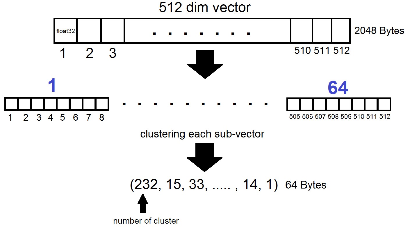
When searching by the vector x, the nearest centroids will be determined first with the usual Flat quantizer, and then x is also divided into sub-vectors, each of which is encoded by the number of one of the 256 corresponding centroids. And the distance to the vector is defined as the sum of 64 distances between sub-vectors.
What is the result?
We stopped our experiments on the index "IVF262144, PQ64", as it fully satisfied all our needs in terms of search speed and accuracy, and also ensured a reasonable use of disk space when further scaling the index. More specifically, at the moment, with 315 million vectors, the index occupies 22 GB of disk space and about 3 GB of RAM when used.
Another interesting detail that we did not mention earlier is the metric used by the index. By default, the distances between any two vectors are calculated in the Euclidean L2 metric, or in more understandable language, the distances are calculated as the square root of the sum of the squares of the coordinate-wise differences. But you can set another metric, in particular, we tested the METRIC_INNER_PRODUCT metric, or metric of cosine distances between vectors. It is cosine because the cosine of the angle between two vectors in the Euclidean coordinate system is expressed as the ratio of the scalar (coordinate-wise) product of vectors to the product of their lengths, and if all vectors in our space have length 1, then the cosine of the angle will be exactly equal to the coordinate-wise product. In this case, the closer the vectors are located in space, the closer to the unit their scalar product will be.
The L2 metric has a direct mathematical transition to the dot product metric. However, when experimentally comparing the two metrics, the impression was that the metric of scalar products helps us analyze the similarity coefficients of images in a more successful way. In addition, the embeddings of our photos were obtained usingInsightFace , which implements the ArcFace architecture using cosine distances. There are also other metrics in FAISS indexes that you can read about here .
a few words about the GPU
FAISS GPU , , , . GPU L2.
, , PQ GPU 56- , float32 float16, .
FAISS GPU , CPU , , GPU . , :
, , PQ GPU 56- , float32 float16, .
FAISS GPU , CPU , , GPU . , :
faiss.omp_set_num_threads(N)Conclusion and curious examples
So, back to where it all began. And it began, recall, with the motivation to solve the problem of finding bots on the Instagram network, and more specifically - to look for duplicate posts with people or avatars in certain sets of users. In the process of writing the material, it became clear that a detailed description of our methodology for searching for bots would require a separate article, which we will discuss in the following publications, but for now we will limit ourselves to examples of our experiments with FAISS.
You can vectorize pictures or faces in different ways, we have chosen the InsightFace technology (vectorizing images and extracting n-dimensional features from them is a separate long story). In the course of experiments with the infrastructure we received, quite interesting and funny properties were discovered.
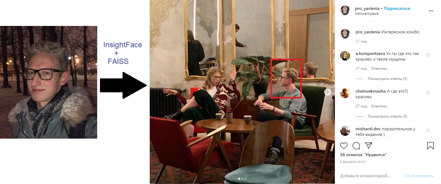
For example, having secured the permission of colleagues and acquaintances, we uploaded their faces into the search and quickly found photographs in which they are present:

Our colleague got into a photo of a Comic-Con visitor, being in the background in a crowd. Source

Picnic in a large company of friends, a photo from a friend’s account. Source

Just passed by. An unknown photographer captured the guys for his thematic profile. They did not know where their photo went, and after 5 years they completely forgot how they were photographed. Source
In this case, the photographer is unknown and photographed secretly!
Immediately recalled the suspicious girl with SLR, sitting at the moment in front of :) Source
Thus, by simple actions FAISS allows you to assemble an analogue of the well-known FindFace on your knee.
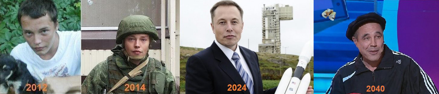
Another interesting feature: in the FAISS index, the more faces resemble each other, the closer the corresponding vectors in space are to each other. I decided to take a closer look at the slightly less accurate search results on my face and found clones terribly similar to myself :)

Some of the author's clones.
Photo Sources: 1 , 2 , 3
Generally speaking, FAISS opens up a huge field for the implementation of any creative ideas. For example, using the same principle of vector proximity of similar faces, one could build paths from one person to another. Or, as a last resort, make a factory for the production of such memes from FAISS:
Source
Thank you for your attention and we hope that this material will be useful to the readers of Habr!
The article was written with the support of my colleagues Artyom Korolev (korolevart), Timur Kadyrov and Arina Reshetnikova.
R&D Dentsu Aegis Network Russia.