 Hello Habitants! Deep learning has become a powerful engine for working with artificial intelligence. Vivid illustrations and simple code examples save you the hassle of delving into the complexities of constructing deep learning models, making complex tasks accessible and fun.
John Krohn, Grant Beileveld, and the illustrator Aglae Bassens, a great illustrator, use vivid examples and analogies to explain what deep learning is, why it is so popular, and how the concept is related to other approaches to machine learning. The book is ideal for developers, data processing specialists, researchers, analysts and novice programmers who want to apply deep learning in their work. The theoretical calculations are perfectly complemented by the application code in Python in Jupyter notebooks. You will learn the techniques for creating effective models in TensorFlow and Keras, as well as get to know PyTorch.
Basic knowledge of deep learning will allow you to create real applications - from computer vision and natural language processing to image generation and game algorithms.
Keras-based intermediate depth network
At the end of this chapter, we will translate the new theoretical knowledge into the neural network and see if we can surpass the previous shallow_net_in_keras.ipynb model in the classification of handwritten numbers.
The first few steps in Jupyter's intermediate_net_in_keras.ipynb notebook are identical to those of its predecessor, the shallow web. First, the same Keras dependencies are loaded, and the MNIST data set is entered and processed in the same way. As you can see in Listing 8.1, the fun part starts where the architecture of the neural network is defined.
Listing 8.1. Code defining the intermediate-depth neural network architecture
model = Sequential()
model.add(Dense(64, activation='relu', input_shape=(784,)))
model.add(Dense(64, activation='relu'))
model.add(Dense(10, activation='softmax'))
The first line in this code snippet, model = Sequential (), is the same as in the previous network (Listing 5.6); This is an instance of a neural network model object. The next line begins the discrepancy. In it, we replaced the activation function sigmoid in the first hidden layer with the relu function, as recommended in Chapter 6. All other parameters of the first layer, except for the activation function, remained the same: it still consists of 64 neurons, and the dimension of the input layer remained the same - 784 neurons.
Another significant change in Listing 8.1 over the shallow architecture in Listing 5.6 is the presence of a second hidden layer of artificial neurons. By calling the model.add () method, we effortlessly add a second Dense layer with 64 relu neurons, justifying the word intermediate in the name of the notepad. By calling model.summary (), you can see, as shown in Fig. 8.9 that this extra layer adds 4160 additional learning parameters, compared to a shallow architecture (see Figure 7.5). Parameters can be divided into:
- 4096 weights corresponding to the connections of each of the 64 neurons in the second hidden layer with each of the 64 neurons in the first hidden layer (64 × 64 = 4096);
- plus 64 offsets, one for each neuron in the second hidden layer;
- the result is 4160 parameters: n parameters = nw + nb = 4096 + 64 =
= 4160.
In addition to the changes in the architecture of the model, we also changed the compilation options for the model, as shown in Listing 8.2.
Listing 8.2. Intermediate Depth Neural Network Compilation Code
model.compile(loss='categorical_crossentropy',
                      optimizer=SGD(lr=0.1),
                      metrics=['accuracy'])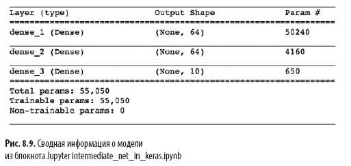
These lines from Listing 8.2:
- set a cost function based on cross entropy: loss = 'categorical_crossentropy' (in a shallow network, the quadratic cost was used loss = 'mean_squared_error');
- set the method of stochastic gradient descent to minimize cost: optimizer = SGD;
- determine the hyperparameter of the learning speed: lr = 0.1 (1) ;
- , , Keras , : metrics=['accuracy'](2).
(1) , , .
(2) , , , , , . , , , . , , : , (, « 86 »), (« 86 , »).
Finally, we train the intermediate network by executing the code in Listing 8.3.
Listing 8.3. Intermediate depth neural network training code
model.fit(X_train, y_train,
              batch_size=128, epochs=20,
              verbose=1,
              validation_data=(X_valid, y_valid))
The only thing that has changed in intermediate network training compared to a shallow network (see Listing 5.7) is a decrease in the order of the epochs hyperparameter from 200 to 20. As you will see later, a more efficient intermediate architecture requires much less epochs to learn.

In fig. 8.10 shows the results of the first four epochs of network training. As you probably remember, our shallow architecture reached a plateau at 86% accuracy on test data after 200 eras. The intermediate depth network significantly surpassed it: as shown by the val_acc field, the network reached 92.34% accuracy after the first training epoch. After the third epoch, accuracy exceeded 95%, and by the 20th epoch it seems to have reached a plateau at about 97.6%. We are seriously moving forward!
Let us examine in more detail the output of model.fit (), shown in Fig. 8.10:
- The
progress bar shown below fills up over 469 “learning cycles” (see Figure 8.5): 60000/60000 [======================== ======] - 1s 15us/step , 469 1 , 15 .
- loss . 0.4744 (SGD) , 0.0332 .
- acc — . 86.37% 99% . , .
- , (val_loss), , 0.08 .
- (val_acc). , 97.6%, 86% .
We have done a great job in this chapter. We first learned how a neural network with fixed parameters processes information. Then we figured out the interacting methods - cost functions, stochastic gradient descent and backpropagation - that allow you to adjust the network parameters to approximate any true y value that has a continuous relationship with some input x. Along the way, we got acquainted with several hyperparameters, including learning rate, packet size and number of learning epochs, as well as the rules of thumb for tuning each of them. At the end of the chapter, we applied our new knowledge to create an intermediate depth neural network, which significantly outperformed the previous shallow network on the same problem of classifying handwritten numbers.Next, we will look at methods to improve the stability of artificial neural networks as they deepen, allowing us to develop and train a full-fledged deep learning model.
»More information about the book can be found on the publisher’s website
» Contents
» Excerpt
For Khabrozhiteley 25% discount on the coupon - Deep learning
Upon the payment of the paper version of the book, an electronic book is sent by e-mail.