The data on more than a million building permits (records in two datasets) from the San Francisco Construction Department allows us to analyze not only the construction activity in the city , but also critically examine the latest trends and development history of the construction industry over the past 40 years , from 1980 to 2019.
Open data makes it possible to study the main factors that have influenced and will influence the development of the construction industry in the city, dividing them into “external” (economic booms and crises) and “internal” (the impact of holidays and seasonal-annual cycles).
Content
Open data and a review of initial parameters.
Annual construction activity in San Francisco.
Expectation and reality in the preparation of the estimated cost.
Construction activity depending on the season of the year.
Total investment in real estate in San Francisco
. Which areas have invested over the past 40 years
?
Statistics on Total Requests by Month and Day
The Future of the San Francisco Construction Industry
Open data and overview of initial parameters.
This is not a translation of the article. I write on LinkedIn and in order not to create charts in several languages - all charts are in English. Link to Jupyter Notebook with data and graphs (for those who are registered on Kaggle - please put plus Notebook - Thank you).
Link to English version: The Ups and Downs of the San Francisco Construction Industry. Trends and History of Construction.
San Francisco building permit data - taken from the open data portal - data.sfgov.org . The portal has several datasets on the construction topic. Two such datasets store and update data on permits issued for the construction or repair of facilities in the city:
- Building permits for the period 1980-2013 (850 thousand entries)
- Building permits for the period after 2013 (280 thousand records, data are downloaded and updated weekly)
These datasets contain information about issued building permits, with various characteristics of the object for which the permit is issued. The total number of records (permits) received in the period 1980-2019 is 1,137,695 permits .

The main parameters from this dataset that were used for analysis:
- permit_creation_date - date of creation of the application (in fact, the day from which construction work begins)
- desctription - description of the application (two or three keywords describing the construction (work) object for which the permit was created)
- estimated_cost - estimated (estimated) cost of construction work
- revised_cost - revised cost (cost of work after revaluation, increase or decrease of the initial volume of the application)
- existing_use - type of housing (one-, two-family house, apartments, offices, production, etc.)
- zipcode, location - zip code and coordinates of the object
Annual building activity in San Francisco
In the graph below, estimated_cost and revised_cost are presented as a distribution of the total cost of work by month.
data_cost_m = data_cost.groupby(pd.Grouper(freq='M')).sum()To reduce monthly “emissions”, monthly data are grouped by year. The graph of the amount of money invested over the years has received a more logical, and amenable to analysis - form.
data_cost_y = data_cost.groupby(pd.Grouper(freq='Y')).sum()
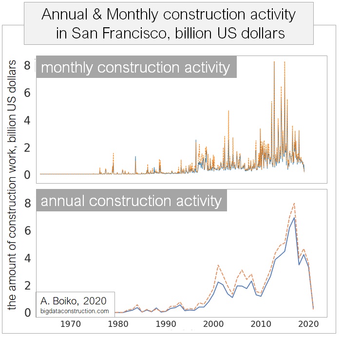
According to the annual movement of the sum of values (all permits for the year) in urban objects , economic factors are clearly visible that, from 1980 to 2019, influenced the number and value of construction projects, or, in other words, on investments in San Francisco real estate.
The number of building permits (the number of construction works or the number of investments) over the past 40 years has been closely related to economic activity in Silicon Valley.

The first peak of construction activity was associated with the electronics hype in the mid-80s in the valley. The ensuing recession in electronics and banking in 1985 left the regional real estate market in decline from which it did not recover for almost a decade.
After that, two more times (in 1993-2000 and 2009-2016) before the collapse of the dot-com bubble and the technological boom of recent years, the construction industry in San Francisco went through a parabolic growth of several thousand percent .
By removing the intermediate peaks and downturns and leaving the minimum and maximum values on each economic cycle, one can see how much large market fluctuations have plagued the industry over the past 40 years.
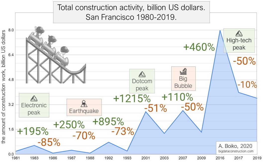
The largest increase in investment in construction came during the dot-com boom, when from 1993 to 2001, $ 10 billion was invested in repairs and construction, or about $ 1 billion a year. If you count in square meters (the cost of 1 m² in 1995 is $ 3,000) - this is approximately 350,000 m2 per year for 10 years, starting in 1993.
The growth of annual total investments for this period amounted to 1215%.
The firms that leased construction equipment during this period were similar to the firms that sold shovels during the gold rush (in the same region in the mid-19th century). Only instead of shovels - in the 2000s there were already cranes and concrete pumps for the newly formed construction companies who wanted to make money on the construction boom.

After each of the many crises that the construction industry has experienced over the years, over the next two post-crisis years, investment (amount of applications for permits) in construction each time fell by at least 50% .
The largest crises in the San Francisco construction industry occurred in the 90s. Where, with a frequency of 5 years, the industry either fell (-85% between 1983-1986), then rose again (+ 895% between 1988-1992), remaining in annual terms in 1981, 1986, 1988, 1993 - on the same level.
After 1993, all subsequent downturns in the construction industry amounted to no more than 50%. But the approaching economic crisis (due to COVID-19) can create a record crisis in the construction industry in the period 2017-2021, the fall of which already for the period 2017-2019 is more than 60% in total.

San Francisco population growth over the period 1980-1993 also showed almost exponential growth... Silicon Valley's economic strength and innovative energy were the solid foundation upon which the hyperbole of the new economy, the American Renaissance, and the dotcoms were built. It was the epicenter of the new economy. But in contrast to the growth in real estate investment, after the peak of dot-coms, the population actually reached a plateau.
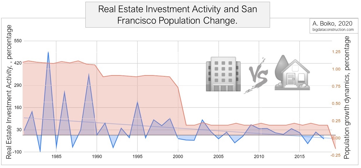
If before the peak of the dotcoms in 2001, since 1950 the annual population growth has been approximately 1% per year. Then, after the collapse of the bubble, the influx of new population has slowed down and since 2001 it has been only 0.2 percent per year.
In 2019 (for the first time since 1950), the growth dynamics showed an outflow of population (-0.21% or 7,000 people) from the city of San Francisco.
Expectation and reality in the preparation of the estimated cost
In the datasets used, the data on the cost of permits for a construction object are divided into:
- initial estimated cost ( estimated_cost )
- cost of work after revaluation ( revised_cost )
During the boom, the main purpose of revaluation is to increase the initial cost, when the investor (construction customer) shows an appetite after the start of construction.
During the crisis, the estimated cost, they try not to exceed, and the initial estimates practically do not undergo changes (with the exception of the 1989 earthquake).
From the graph plotted on the difference between the revalued and estimated cost (revised_cost - estimated_cost), you can observe that:
The amount of cost increase during the revaluation of the volume of construction work - directly depends on the cycles of the economic boom
data_spread = data_cost.assign(spread = (data_cost.revised_cost-data_cost.estimated_cost))
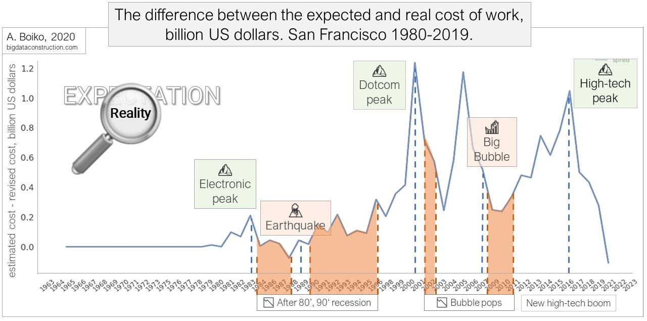
During periods of rapid economic growth, work customers (investors) spend their money generously enough, increasing their requests after the work starts.
The client (investor), feeling financially secure, asks the building contractor or architect to extend the already issued building permit. This may be a decision to increase the initial length of the pool or increase the area of the house (after the start of work and the issuance of a building permit).
At the peak of dotcoms, such “additional” expenses reached the “extra” 1 billion per year.

If you look at this table already in percentage change, then the peak increase in estimates (100% or 2 times the initial estimated cost) came in the year before the earthquake in 1989 near the city. I suppose that after the earthquake, the construction projects that were started in 1988 required more time and money for implementation after the earthquake in 1989.
Conversely, a downward revision of the estimated cost (which happened only once from 1980 to 2019) a few years before the earthquake, presumably due to the fact that some objects started in 1986-1987 were frozen or investments in these objects have been curtailed. On scheduleon average, for each object begun in 1987 - the estimated cost reduction was -20% of the original plan .
data_spred_percent = data_cost_y.assign(spred = ((data_cost_y.revised_cost-data_cost_y.estimated_cost)/data_cost_y.estimated_cost*100))
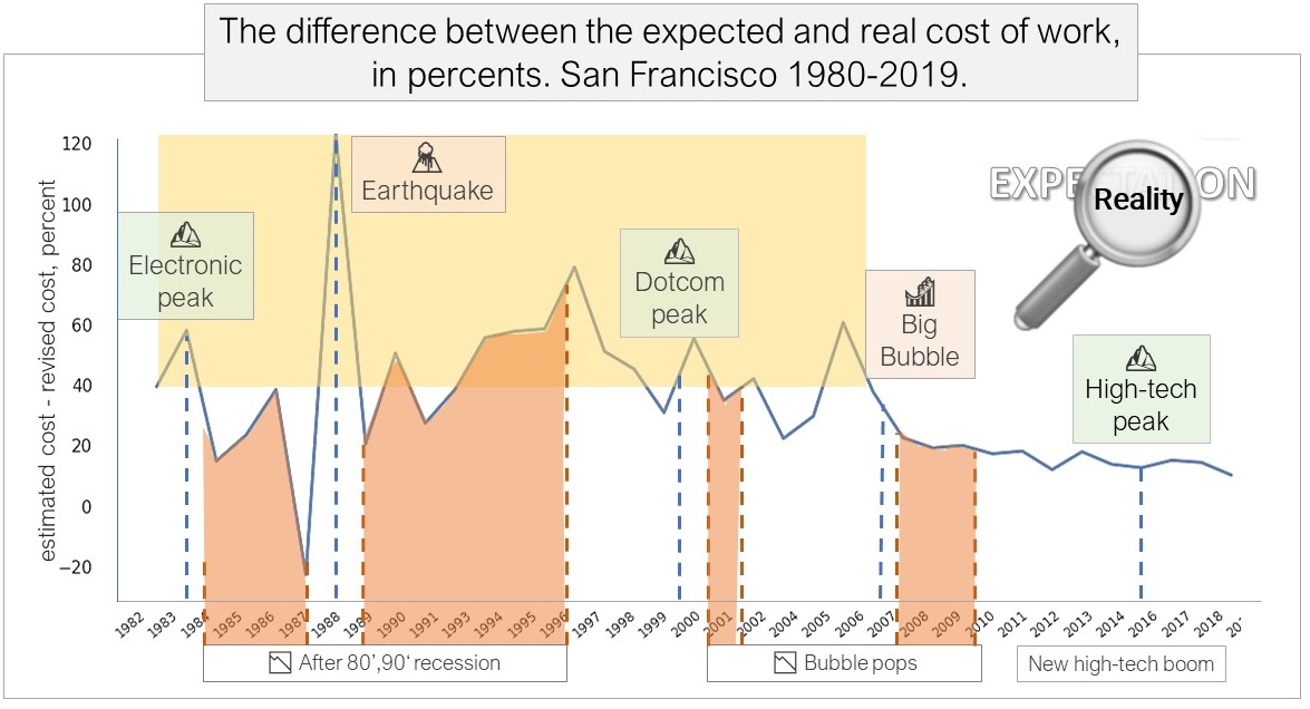
An increase in the initial estimated cost by more than 40% indicated or was possibly the result of an approaching bubble in the financial and subsequently construction market.
What is the reason for the decrease in the spread (difference) between the estimated and revised value after 2007?
Perhaps investors began to carefully look at the numbers (the average amount over 20 years increased from $ 100 thousand to $ 2 million) or perhaps the construction department, warning and slowing down the emerging bubbles in the real estate market, introduced new rules and restrictions to reduce possible manipulations and possible risks that will arise during the crisis years.
Construction activity depending on the season of the year
By grouping the data by calendar weeks in a year (54 weeks), you can observe the construction activity of the city of San Francisco depending on the seasonality and time of year.
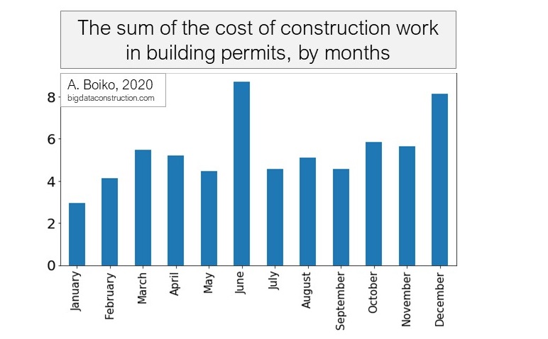
By Christmas, all construction organizations are trying to have time to get permission for new "large" objects (at the same time! The number! Of permits in the same months is at the same level throughout the year). Investors, planning to receive their object within the next year, conclude contracts in the winter months, counting on large discounts (since summer contracts, for the most part, come to an end by the end of the year and construction firms are interested in receiving new applications).
Before Christmas, the largest amounts are filed in applications (an increase from an average of 1-1.5 billion per month. To 5 billion in December alone).At the same time, the total number of applications by month remains at the same level (see section below: statistics on the total number of applications by months and days)
After the winter holidays, the construction industry is actively (almost without an increase in the number of permits) planning and implementing “Christmas” orders in order to by the middle of the year (before the holiday “Independence Day”) - to have time to free up resources before starting a new wave of summer agreements beginning immediately after the June holidays.
data_month_year = data_month_year.assign(week_year = data_month_year.permit_creation_date.dt.week)
data_month_year = data_month_year.groupby(['week_year'])['estimated_cost'].sum()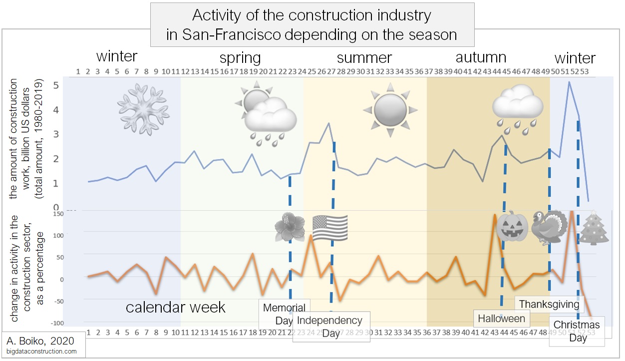
The same percentage data (orange line) also shows that the industry works “smoothly” throughout the year, but before and after the holidays, the activity on permits increases to 150% in the period between week 20-24 (before Independence Day), and decreases immediately after the holiday up to -70%.
Before Halloween and Christmas, activity in the construction industry in San Francisco during week 43-44 increases by 150% (from bottom to peak) and then decreases to zero during the holidays.
Thus, the industry is in a semi-annual cycle, which is separated by the holidays "US Independence Day" (week 20) and "Christmas" (week 52).
Total investment in San Francisco real estate
Based on the data on building permits in the city:
Total investment in San Francisco construction projects between 1980 and 2019 is $ 91.5 billion.
sf_worth = data_location_lang_long.cost.sum()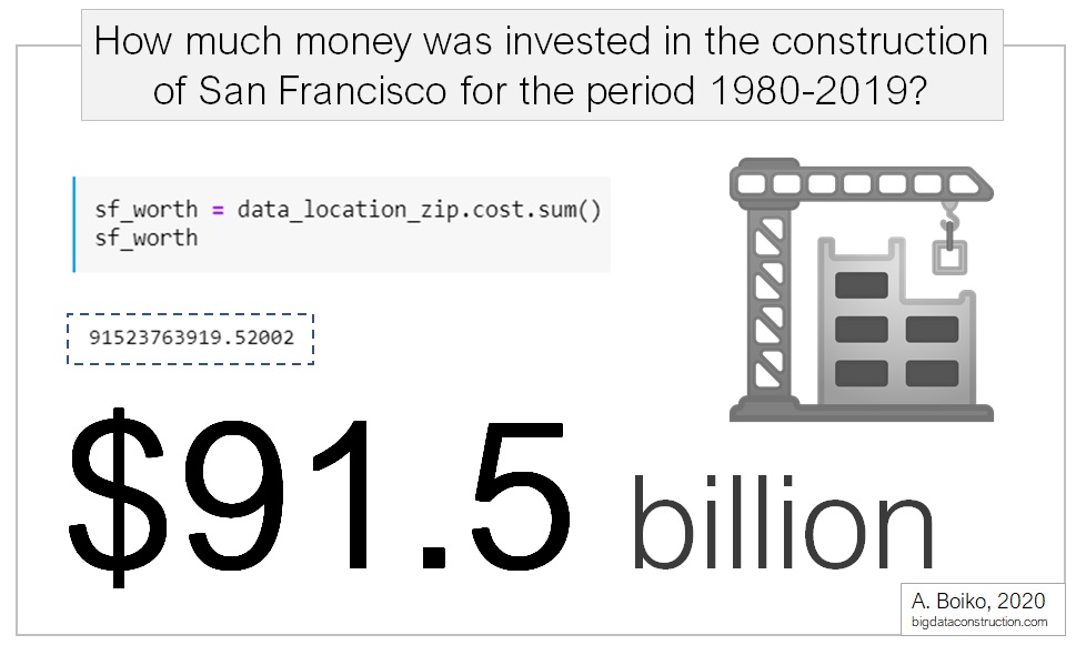
The total market value of all residential real estate in San Francisco, estimated by property tax (is the estimated value of all real estate and all personal property owned by San Francisco) reached $ 208 billion in 2016 .
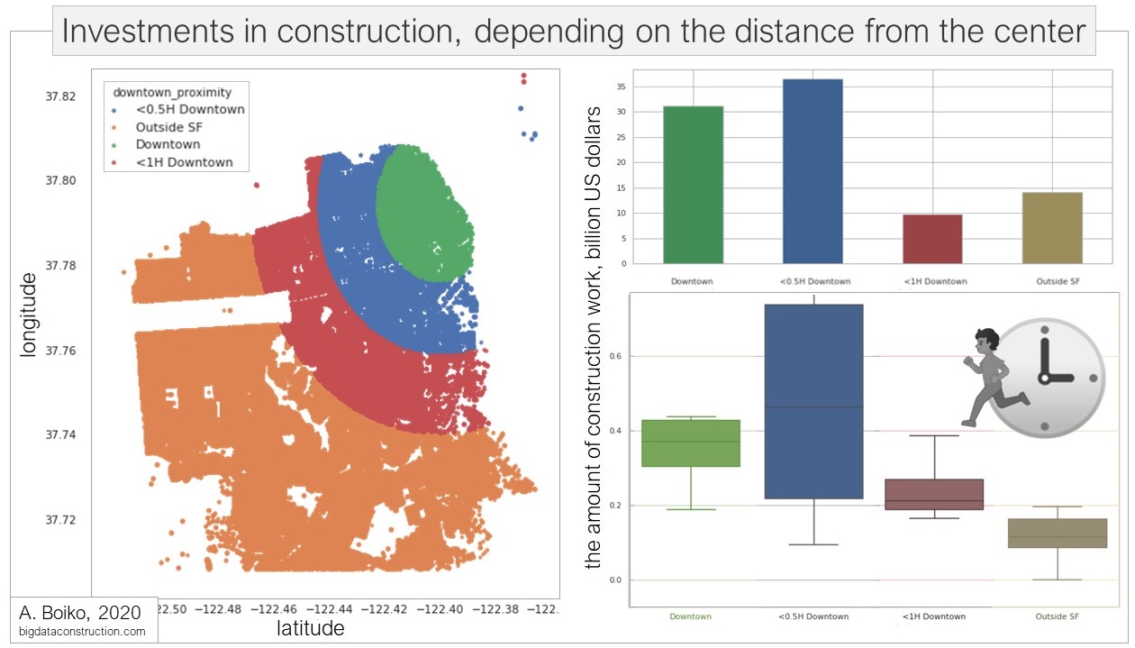
In which areas of San Francisco have invested over the past 40 years
With the help of the Folium library, let's see where these $ 91.5 billion by regions were invested. To do this, grouping the data by zip code (zipcode), imagine the value obtained using circles (Circle function from the Folium library).
import folium
from folium import Circle
from folium import Marker
from folium.features import DivIcon

# map folium display
lat = data_location_lang_long.lat.mean()
long = data_location_lang_long.long.mean()
map1 = folium.Map(location = [lat, long], zoom_start = 12)

for i in range(0,len(data_location_lang_long)):
    Circle(
        location = [data_location_lang_long.iloc[i]['lat'], data_location_lang_long.iloc[i]['long']],
        radius= [data_location_lang_long.iloc[i]['cost']/20000000],
        fill = True, fill_color='#cc0000',color='#cc0000').add_to(map1)
    Marker(
    [data_location_mean.iloc[i]['lat'], data_location_mean.iloc[i]['long']],
    icon=DivIcon(
        icon_size=(6000,3336),
        icon_anchor=(0,0),
        html='<div style="font-size: 14pt; text-shadow: 0 0 10px #fff, 0 0 10px #fff;; color: #000";"">%s</div>'
        %("$ "+ str((data_location_lang_long.iloc[i]['cost']/1000000000).round()) + ' mlrd.'))).add_to(map1)
map1


In the districts, it is clear that the majority of the pie went to DownTown. Having simplified the grouping of all objects according to the distance to the city center and the time needed to get to the city center (of course, expensive houses are also being built on the coast), all permissions were divided into 4 groups: 'Downtown', '<0.5H Downtown', '< 1H Downtown ',' Outside SF '.
from geopy.distance import vincenty
def distance_calc (row):
    start = (row['lat'], row['long'])
    stop = (37.7945742, -122.3999445)

    return vincenty(start, stop).meters/1000

df_pr['distance'] = df_pr.apply (lambda row: distance_calc (row),axis=1)

def downtown_proximity(dist):
    '''
    < 2 -> Near Downtown,  >= 2, <4 -> <0.5H Downtown
    >= 4, <6 -> <1H Downtown, >= 8 -> Outside SF
    '''
    if dist < 2:
        return 'Downtown'
    elif dist < 4:
        return  '<0.5H Downtown'
    elif dist < 6:
        return '<1H Downtown'
    elif dist >= 6:
        return 'Outside SF'
df_pr['downtown_proximity'] = df_pr.distance.apply(downtown_proximity)
Of the 91.5 billion invested in the city, almost 70 billion (75% of all investments) invested in repair and construction are in the city center (green zone) and in the city area within a radius of 2 km. from the center (blue zone).
Average estimated cost of a construction application by city districts
All data, as in the case of the total investment, was grouped by postal code. Only in this case, with the average (.mean ()) estimated cost of the application by postal code.
data_location_mean = data_location.groupby(['zipcode'])['lat','long','estimated_cost'].mean()
In ordinary areas of the city (more than 2 km from the city center) - the average estimated cost of the application for construction is $ 50 thousand.

The average estimated cost in the city center area is about three times higher ($ 150 thousand to $ 400 thousand) than other areas ($ 30-50 thousand).
Apart from the cost of land, three factors determine the total cost of housing construction: labor, materials, and government fees. These three components are higher in California than in the rest of the country. California's building codes and standards are considered among the most comprehensive and stringent in the nation (due to earthquakes and environmental regulations), often requiring more expensive materials and labor.
For example, the government requires builders to use higher quality building materials (windows, insulation, heating and cooling systems) in order to achieve high energy efficiency standards.

From the general statistics on the average cost of an application for a permit, two locations are knocked out:
- Treasure Island is an artificial island in the San Francisco Bay. The average estimated cost of a building permit is $ 6.5 million.
- Mission Bay - (2,926 residents) Estimated average cost of a building permit - $ 1.5 million.

In fact, the high average bid in these two regions is associated with the smallest number of bids for these postal locations (145 and 3064, respectively, construction on the island is very limited), while for the rest of the postal codes - for the period 1980-2019, about 1300 were received applications per year (in total, an average of 30-50 thousand applications for the entire period).
By the parameter “number of applications”, a perfectly even distribution of the number of applications per one zip code is noticeable throughout the city.
Statistics on the total number of applications by month and day
Overall statistics on the total number of applications by month and day of the week from 1980 to 2019 show that the “quietest” months for the building department are the spring and winter months. Moreover, the amount of investments indicated in the applications varies greatly, and differs significantly from month to month (see in addition, “Construction activity depending on the season of the year”). Among the days of the week on Monday, the department’s workload is approximately 20% less than the rest of the week.
months = [ 'January', 'February', 'March', 'April', 'May','June', 'July', 'August', 'September', 'October', 'November', 'December' ]
data_month_count  = data_month.groupby(['permit_creation_date']).count().reindex(months)

While June and July practically do not differ in the number of applications, in the total estimated cost the difference reaches 100% (4.3 billion in May and July and 8.2 billion in June).
data_month_sum = data_month.groupby(['permit_creation_date']).sum().reindex(months)
The future of the San Francisco construction industry, predicting activity by patterns.
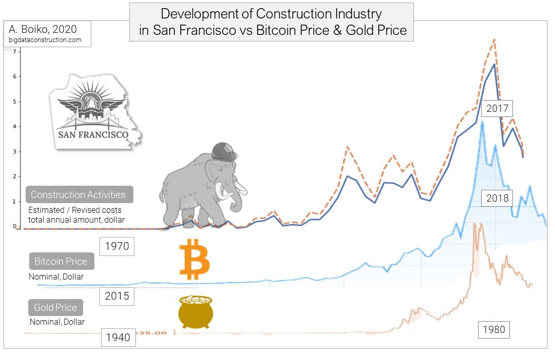
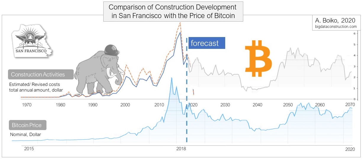
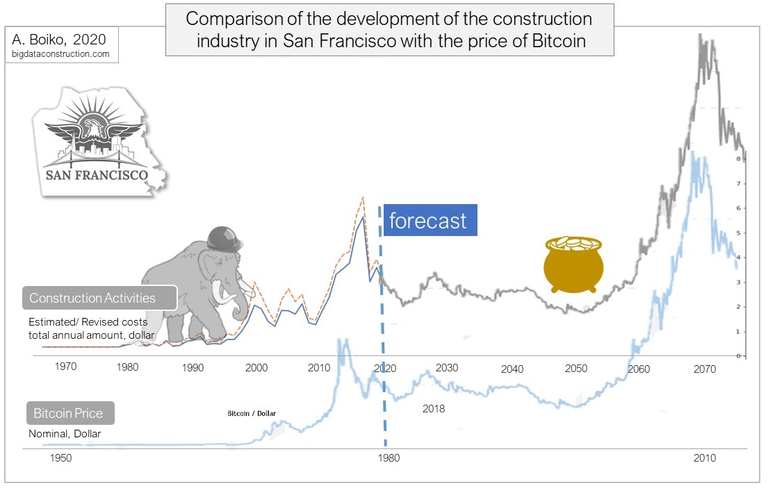
In conclusion, we compare the graph of construction activity in San Francisco with the graph of Bitcoin prices (2015-2018) and the graph of gold prices (1940 - 1980).
Pattern (from the English pattern - model, sample) - in the technical analysis are called persistent repetitive combinations of price, volume, or indicator data. Pattern analysis is based on one of the axioms of technical analysis: “history repeats itself” - it is believed that repeated combinations of data lead to a similar result.
The main pattern that can be guessed on the annual activity chart is “Head and Shoulders” - a trend reversal pattern.It is so named because the graph looks like a human head (peak) and shoulders on the sides (smaller peaks). When the price breaks the line connecting the troughs, the pattern is considered complete and the move is likely to be downward.
The movement of activity in the construction industry of San Francisco almost completely coincides with the graph of the growth of the price of gold and bitcoin. The historical performance of these three charts of price movement and activity shows marked similarities.
In order to be able to predict the behavior of the construction market in the future, it is necessary to calculate the correlation coefficient with each of these two trends.
Two random variables are called correlated if their correlation moment (or correlation coefficient) is different from zero; and are called uncorrelated quantities if their correlation moment is zero.
If the obtained value is closer to 0 than to 1, then talking about a clear pattern does not make sense. This is a difficult mathematical problem, which senior comrades may possibly take on, who may be interested in this topic.
If a! unscientific! look at the topic of further development of the construction industry in San Francisco: if the pattern matches further with the price of bitcoin, thenaccording to this pessimistic option , coming out of the crisis in the construction industry in San Francisco will not be easy for the near post-crisis time.
In a more “optimistic” scenario, a repeated exponential growth of the construction industry is possible if activity here follows the “gold price” scenario. In this option, in 20-30 years (maybe in 10), the construction sector expects a new surge in employment and development.
In the next part, I will take a closer look at individual sectors of construction (repair of roofs, kitchens, construction of stairs, bathrooms, if you have wishes for industries or other data - please write in the comments) and compare inflation for certain types of work with a fixed rate on mortgage loans and the yield on US government bonds (Fixed Mortgage Rates & US Treasury Yield).
Link to Jupyter Notebook: San Francisco. Building sector 1980-2019.
Please, for those with Kaggle - put plus Notebook (Thank you!).
(Comments and explanations of the code will be added to the Notebook later)
Link to the English version: The Ups and Downs of the San Francisco Construction Industry. Trends and History of Construction.
If you like my content, please consider buying me a coffee.
thanks for your support!
Buy coffee for the author