
We will take as a basis the scripts from Appendix B - Greek Mythology Graph Example of the SAP HANA Graph Reference documentation for a typical SAP HANA platform that is deployed locally in the data center. The main purpose of this example is to show the analytical capabilities of SAP HANA, to show how you can analyze the relationship between objects and events using graph algorithms. We will not dwell on this technology in detail, the main idea will be clear from the further presentation. Those who are interested can figure it out on their own, having experienced the capabilities of SAP HANA express edition or take a free course Analyzing Connected Data with SAP HANA Graph .
Let's put the data in the SAP HANA Cloud relational cloud and see the possibilities for analyzing the family ties of Greek heroes. Remember, in “Myths and Legends of Ancient Greece” there were a lot of characters and by the middle you don’t remember who the son and brother of whom? Here we will make a memo to ourselves and will never forget.
First, let's create an instance of SAP HANA Cloud. This is quite simple to do, you need to fill in the parameters of the future system and wait a few minutes until the instance is deployed for you (Fig. 1).

Figure 1
So, click the Create Instance button and the first page of the creation wizard opens in front of us, on which you need to specify a short name for the instance, set a password and provide a description (Figure 2)
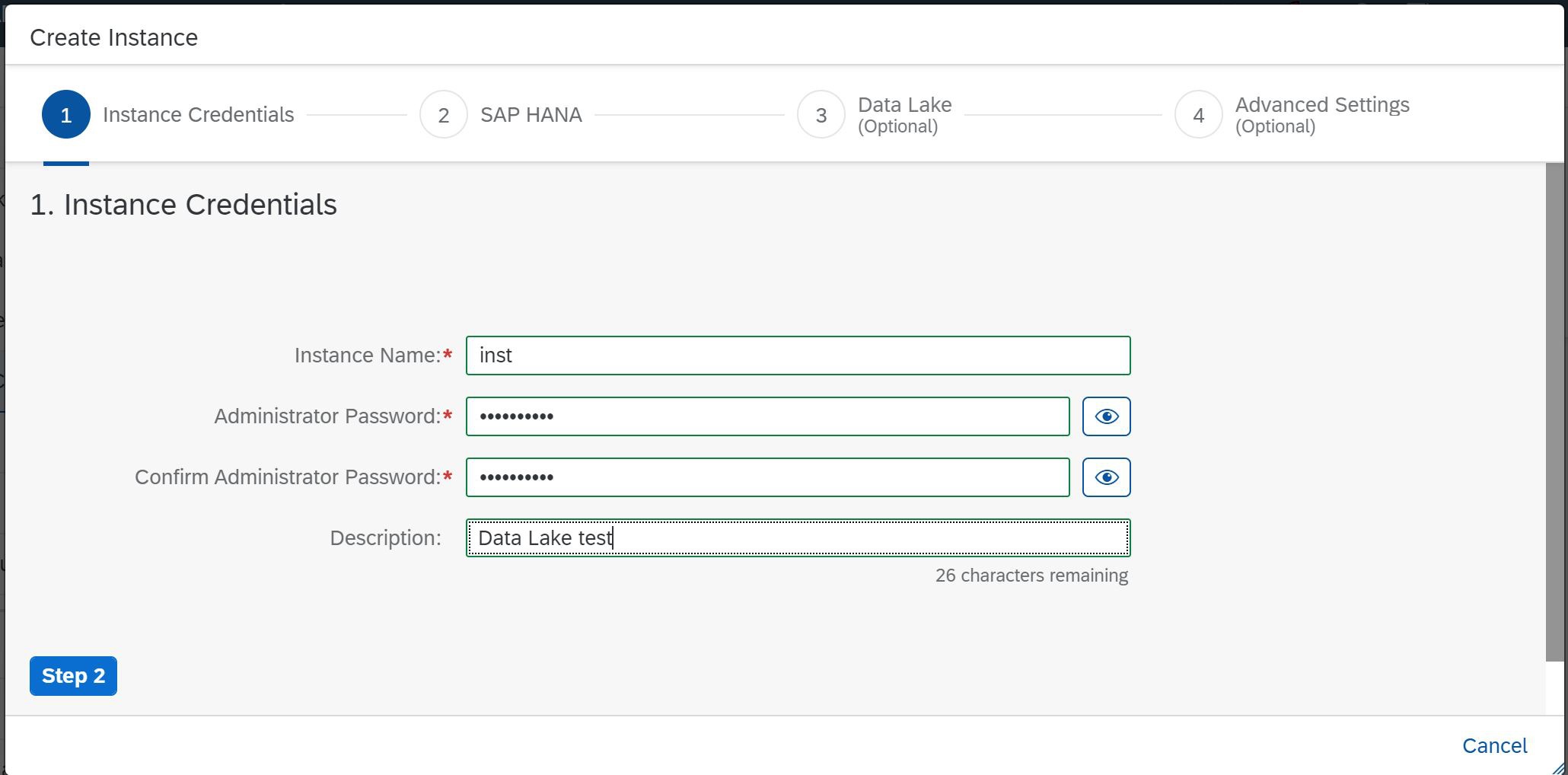
Figure 2
We click the Step 2 button, now our task is to specify the parameters of the future SAP HANA instance. Here you can set only the size of the RAM of the future system, all other parameters will be determined automatically (Fig. 3).

Figure 3
We see that now we have the opportunity to choose the minimum value of 30GB and the maximum value of 900GB. We select 30 GB and it is automatically determined that with this amount of memory, two virtual processors are needed to support calculations and 120 GB to store data on disk. More space is allocated here, since we can use the SAP HANA Native Storage Extension (NSE) technology. If you choose a larger memory size, for example, 255GB, you will need 17 virtual processors and 720GB of disk memory (Fig. 4).
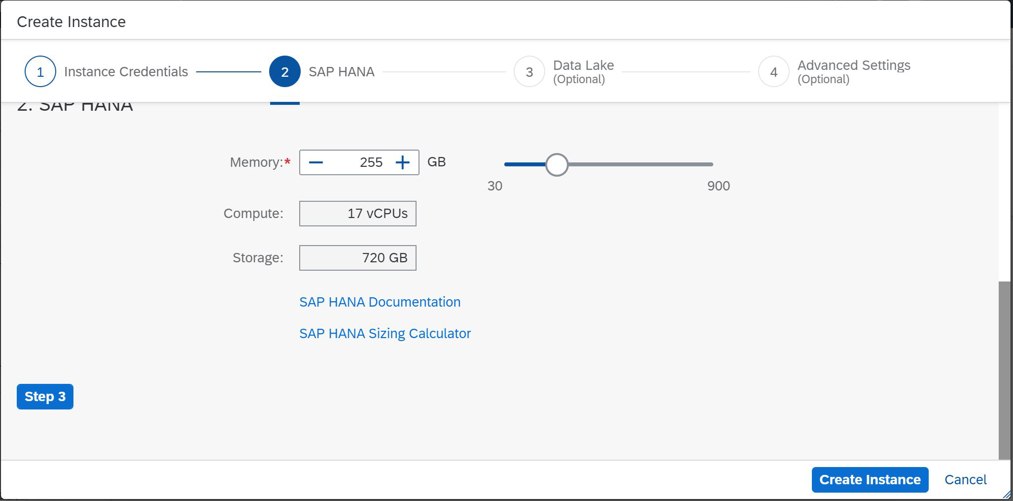
Figure 4
But we don't need so much memory for the example. We return the parameters to their original values and click Step 3. Now we must choose whether to use the data lake. The answer is obvious to us. Sure, we will. We also want to conduct such an experiment (Fig. 5).

Figure 5
At this step, we have much more opportunities and freedom to create an instance of the data lake. You can choose the size of the required computing resources and disk storage. The parameters of the used components / nodes are selected automatically. The system will itself determine the necessary computing resources for the "coordinator" and "working" nodes. If you would like to learn more about these components, then it is better to turn to SAP IQ resources and SAP HANA Cloud data lake.... And we move on, click Step 4.
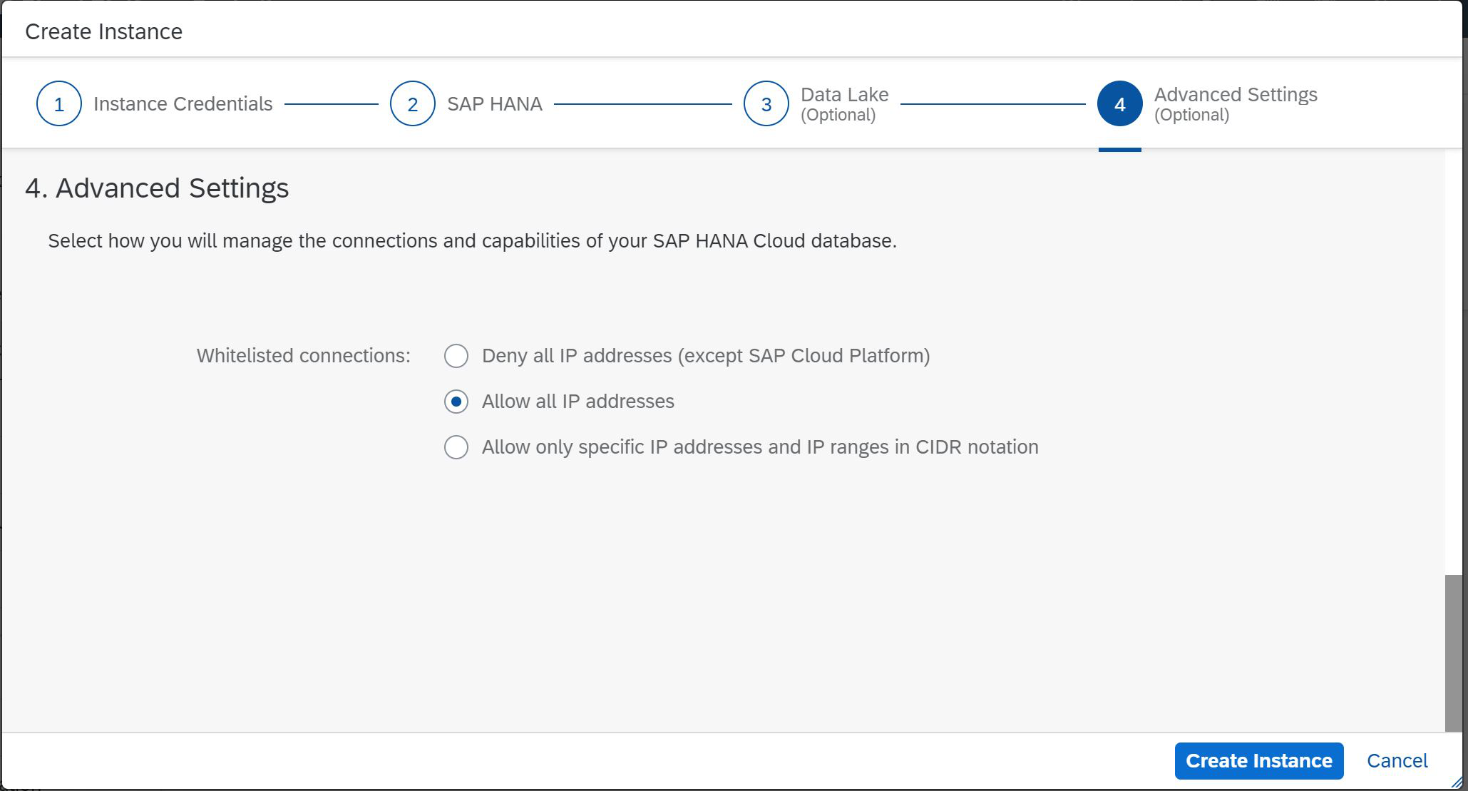
Figure 6
In this step, we will define or restrict the IP addresses that can access the future SAP HANA instance. As you can see, this is the last step of our master (Fig. 6), it remains to click Create Instance and go to pour yourself coffee.

Figure 7
The process has started (Figure 7) and it won't take much time, we just had time to drink strong coffee, despite the late night. And when else can you safely experiment with the system and fasten different chips? So, our system is created (Fig. 8).

Figure 8
We have two options: open SAP HANA Cockpit or SAP HANA Database Explorer. We know that the second product can be launched from Cockpit. Therefore, we open the SAP HANA Cockpit, at the same time and see what is there. But first, you will need to provide a user and his password. Please note that the SYSTEM user is not available to you; you must use DBADMIN. At the same time, specify the password that you set when creating the instance, as in Fig. 9.
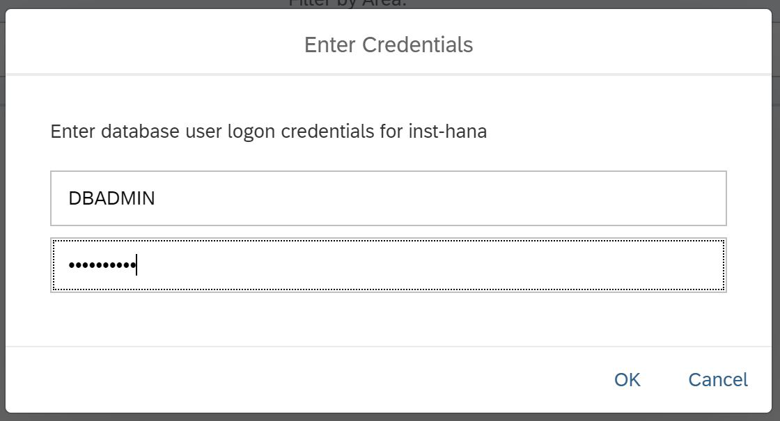
Figure 9
We entered Cockpit and see the traditional SAP interface in the form of tiles, when each of them is responsible for its own task. In the upper right corner we see a link to the SQL Console (Fig. 10).
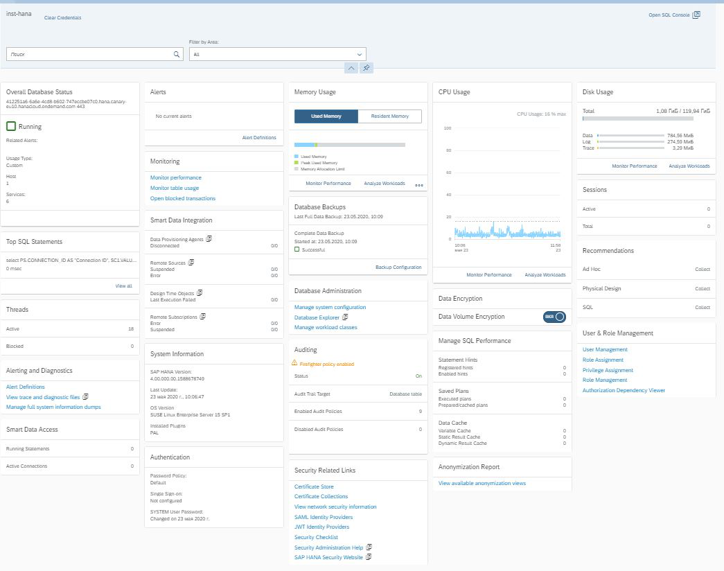
Figure 10
It is she who allows us to go to the SAP HANA Database Explorer.
The interface of this tool is similar to the SAP Web IDE, but is intended only for working with database objects. First of all, of course, we are interested in how to get into the data lake. After all, now we have opened a tool for working with HANA. We’ll go to the Remote Source item in the navigator and see a link to the lake (SYSRDL, RDL - Relation Data Lake). This is the desired access (Fig. 11).
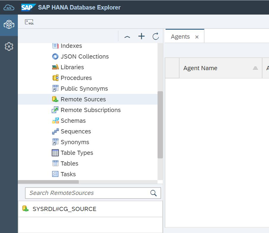
Figure 11
Moving on, we don't have to work under an administrator. We need to create a test user, under which we will experiment with the HANA graph engine, but place the data in a relational data lake.
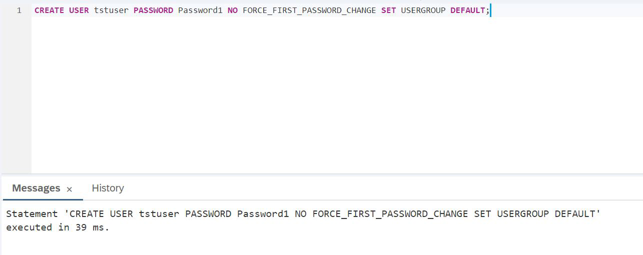
SCRIPT:
CREATE USER tstuser PASSWORD Password1 NO FORCE_FIRST_PASSWORD_CHANGE SET USERGROUP DEFAULT;We plan to work with the data lake, so it is imperative to give rights, for example, HANA_SYSRDL # CG_ADMIN_ROLE, so that you can freely create objects, do whatever we want.
SCRIPT:
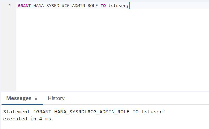
GRANT HANA_SYSRDL#CG_ADMIN_ROLE TO tstuser;Now the work under the SAP HANA administrator is completed, SAP HANA Database Explorer can be closed and we need to log in under the new user created: tstuser. For simplicity, let's go back to the SAP HANA Cockpit and end the admin session. To do this, in the upper left corner there is such a link Clear Credentials (Fig. 12).

Figure 12
After clicking on it, we need to log in again, but now under the user tstuser (Fig. 13).
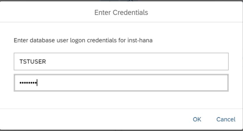
Figure 13
And we can open the SQL Console again to return to SAP HANA Database Explorer, but under a new user (Figure 14).

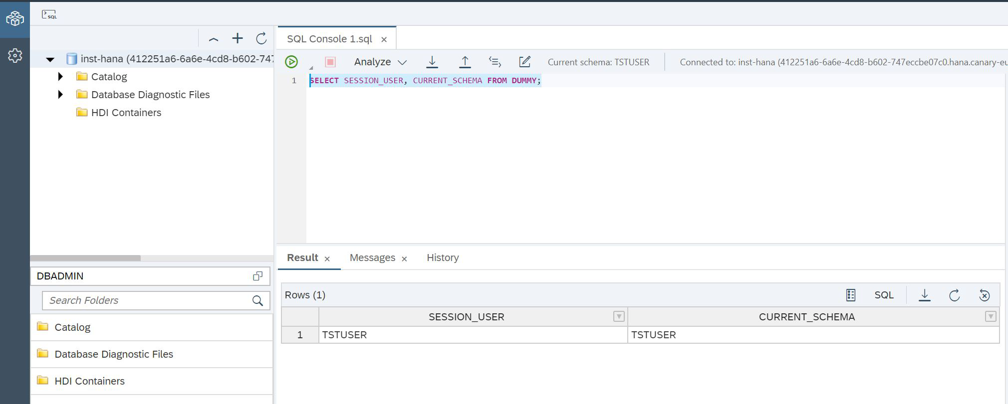
Figure 14
SCRIPT:
SELECT SESSION_USER, CURRENT_SCHEMA FROM DUMMY;That's it, now we are sure that we are working with HANA under the right user. It's time to create tables in the data lake. To do this, there is a special procedure SYSRDL # CG.REMOTE_EXECUTE, into which you need to pass one parameter - a line = command. Using this function, we create a table in the data lake (Fig. 15), in which all our characters will be stored: heroes, Greek Gods and titans.

Figure 15
SCRIPT:
CALL SYSRDL#CG.REMOTE_EXECUTE ('
BEGIN

	CREATE TABLE "MEMBERS" (
		"NAME"       VARCHAR(100) PRIMARY KEY,
		"TYPE"       VARCHAR(100),
		"RESIDENCE"  VARCHAR(100)
	);


END');
And then we create a table in which we will store the relationships of these characters (Fig. 16).

Figure 16
SCRIPT:
CALL SYSRDL#CG.REMOTE_EXECUTE ('
BEGIN
	CREATE TABLE "RELATIONSHIPS" (
		"KEY"    INTEGER UNIQUE NOT NULL,
		"SOURCE" VARCHAR(100) NOT NULL,
		"TARGET" VARCHAR(100) NOT NULL,
		"TYPE"   VARCHAR(100),
		FOREIGN KEY RELATION_SOURCE ("SOURCE") references "MEMBERS"("NAME") ON UPDATE RESTRICT ON DELETE RESTRICT,
		FOREIGN KEY RELATION_TARGET ("TARGET") references "MEMBERS"("NAME") ON UPDATE RESTRICT ON DELETE RESTRICT
	);
END');
We will not deal with integration issues now, this is a separate story. In the original example, there are INSERT commands for creating the Greek Gods and their kinship. We use these commands. We just need to remember that we are passing the command through a procedure to the data lake, so we need to double the quotes, as shown in Fig. 17.

Figure 17
SCRIPT:
CALL SYSRDL#CG.REMOTE_EXECUTE ('
BEGIN
	INSERT INTO "MEMBERS"("NAME", "TYPE")
    	VALUES (''Chaos'', ''primordial deity'');
	INSERT INTO "MEMBERS"("NAME", "TYPE")
    	VALUES (''Gaia'', ''primordial deity'');
	INSERT INTO "MEMBERS"("NAME", "TYPE")
    	VALUES (''Uranus'', ''primordial deity'');
	INSERT INTO "MEMBERS"("NAME", "TYPE", "RESIDENCE")
    	VALUES (''Rhea'', ''titan'', ''Tartarus'');
	INSERT INTO "MEMBERS"("NAME", "TYPE", "RESIDENCE")
    	VALUES (''Cronus'', ''titan'', ''Tartarus'');
	INSERT INTO "MEMBERS"("NAME", "TYPE", "RESIDENCE")
    	VALUES (''Zeus'', ''god'', ''Olympus'');
	INSERT INTO "MEMBERS"("NAME", "TYPE", "RESIDENCE")
    	VALUES (''Poseidon'', ''god'', ''Olympus'');
	INSERT INTO "MEMBERS"("NAME", "TYPE", "RESIDENCE")
    	VALUES (''Hades'', ''god'', ''Underworld'');
	INSERT INTO "MEMBERS"("NAME", "TYPE", "RESIDENCE")
    	VALUES (''Hera'', ''god'', ''Olympus'');
	INSERT INTO "MEMBERS"("NAME", "TYPE", "RESIDENCE")
    	VALUES (''Demeter'', ''god'', ''Olympus'');
	INSERT INTO "MEMBERS"("NAME", "TYPE", "RESIDENCE")
    	VALUES (''Athena'', ''god'', ''Olympus'');
	INSERT INTO "MEMBERS"("NAME", "TYPE", "RESIDENCE")
    	VALUES (''Ares'', ''god'', ''Olympus'');
	INSERT INTO "MEMBERS"("NAME", "TYPE", "RESIDENCE")
    	VALUES (''Aphrodite'', ''god'', ''Olympus'');
	INSERT INTO "MEMBERS"("NAME", "TYPE", "RESIDENCE")
    	VALUES (''Hephaestus'', ''god'', ''Olympus'');
	INSERT INTO "MEMBERS"("NAME", "TYPE", "RESIDENCE")
    	VALUES (''Persephone'', ''god'', ''Underworld'');
END');
And the second table (Fig. 18)
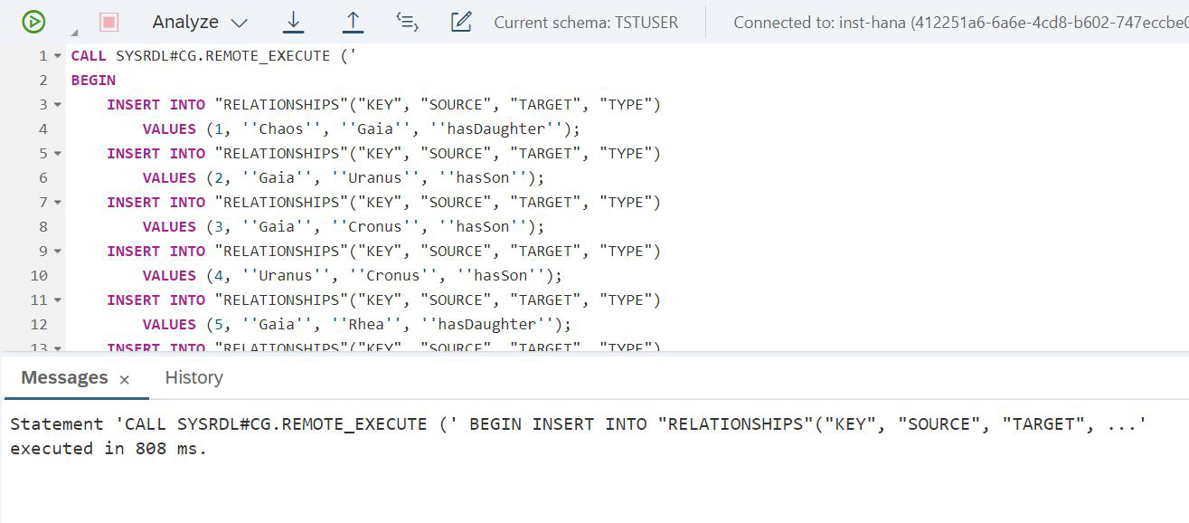
Figure 18
SCRIPT:
CALL SYSRDL#CG.REMOTE_EXECUTE ('
BEGIN
	INSERT INTO "RELATIONSHIPS"("KEY", "SOURCE", "TARGET", "TYPE")
    	VALUES (1, ''Chaos'', ''Gaia'', ''hasDaughter'');
	INSERT INTO "RELATIONSHIPS"("KEY", "SOURCE", "TARGET", "TYPE")
    	VALUES (2, ''Gaia'', ''Uranus'', ''hasSon'');
	INSERT INTO "RELATIONSHIPS"("KEY", "SOURCE", "TARGET", "TYPE")
    	VALUES (3, ''Gaia'', ''Cronus'', ''hasSon'');
	INSERT INTO "RELATIONSHIPS"("KEY", "SOURCE", "TARGET", "TYPE")
    	VALUES (4, ''Uranus'', ''Cronus'', ''hasSon'');
	INSERT INTO "RELATIONSHIPS"("KEY", "SOURCE", "TARGET", "TYPE")
    	VALUES (5, ''Gaia'', ''Rhea'', ''hasDaughter'');
	INSERT INTO "RELATIONSHIPS"("KEY", "SOURCE", "TARGET", "TYPE")
    VALUES (6, ''Uranus'', ''Rhea'', ''hasDaughter'');
INSERT INTO "RELATIONSHIPS"("KEY", "SOURCE", "TARGET", "TYPE")
    VALUES (7, ''Cronus'', ''Zeus'', ''hasSon'');
INSERT INTO "RELATIONSHIPS"("KEY", "SOURCE", "TARGET", "TYPE")
    VALUES (8, ''Rhea'', ''Zeus'', ''hasSon'');
INSERT INTO "RELATIONSHIPS"("KEY", "SOURCE", "TARGET", "TYPE")
    VALUES (9, ''Cronus'', ''Hera'', ''hasDaughter'');
INSERT INTO "RELATIONSHIPS"("KEY", "SOURCE", "TARGET", "TYPE")
    VALUES (10, ''Rhea'', ''Hera'', ''hasDaughter'');
INSERT INTO "RELATIONSHIPS"("KEY", "SOURCE", "TARGET", "TYPE")
    VALUES (11, ''Cronus'', ''Demeter'', ''hasDaughter'');
INSERT INTO "RELATIONSHIPS"("KEY", "SOURCE", "TARGET", "TYPE")
    VALUES (12, ''Rhea'', ''Demeter'', ''hasDaughter'');
INSERT INTO "RELATIONSHIPS"("KEY", "SOURCE", "TARGET", "TYPE")
    VALUES (13, ''Cronus'', ''Poseidon'', ''hasSon'');
INSERT INTO "RELATIONSHIPS"("KEY", "SOURCE", "TARGET", "TYPE")
    VALUES (14, ''Rhea'', ''Poseidon'', ''hasSon'');
INSERT INTO "RELATIONSHIPS"("KEY", "SOURCE", "TARGET", "TYPE")
    VALUES (15, ''Cronus'', ''Hades'', ''hasSon'');
INSERT INTO "RELATIONSHIPS"("KEY", "SOURCE", "TARGET", "TYPE")
    VALUES (16, ''Rhea'', ''Hades'', ''hasSon'');
INSERT INTO "RELATIONSHIPS"("KEY", "SOURCE", "TARGET", "TYPE")
    VALUES (17, ''Zeus'', ''Athena'', ''hasDaughter'');
INSERT INTO "RELATIONSHIPS"("KEY", "SOURCE", "TARGET", "TYPE")
    VALUES (18, ''Zeus'', ''Ares'', ''hasSon'');
INSERT INTO "RELATIONSHIPS"("KEY", "SOURCE", "TARGET", "TYPE")
    VALUES (19, ''Hera'', ''Ares'', ''hasSon'');
INSERT INTO "RELATIONSHIPS"("KEY", "SOURCE", "TARGET", "TYPE")
    VALUES (20, ''Uranus'', ''Aphrodite'', ''hasDaughter'');
INSERT INTO "RELATIONSHIPS"("KEY", "SOURCE", "TARGET", "TYPE")
    VALUES (21, ''Zeus'', ''Hephaestus'', ''hasSon'');
INSERT INTO "RELATIONSHIPS"("KEY", "SOURCE", "TARGET", "TYPE")
    VALUES (22, ''Hera'', ''Hephaestus'', ''hasSon'');
INSERT INTO "RELATIONSHIPS"("KEY", "SOURCE", "TARGET", "TYPE")
    VALUES (23, ''Zeus'', ''Persephone'', ''hasDaughter'');
INSERT INTO "RELATIONSHIPS"("KEY", "SOURCE", "TARGET", "TYPE")
    VALUES (24, ''Demeter'', ''Persephone'', ''hasDaughter'');
INSERT INTO "RELATIONSHIPS"("KEY", "SOURCE", "TARGET", "TYPE")
    VALUES (25, ''Zeus'', ''Hera'', ''marriedTo'');
INSERT INTO "RELATIONSHIPS"("KEY", "SOURCE", "TARGET", "TYPE")
    VALUES (26, ''Hera'', ''Zeus'', ''marriedTo'');
INSERT INTO "RELATIONSHIPS"("KEY", "SOURCE", "TARGET", "TYPE")
    VALUES (27, ''Hades'', ''Persephone'', ''marriedTo'');
INSERT INTO "RELATIONSHIPS"("KEY", "SOURCE", "TARGET", "TYPE")
    VALUES (28, ''Persephone'', ''Hades'', ''marriedTo'');
INSERT INTO "RELATIONSHIPS"("KEY", "SOURCE", "TARGET", "TYPE")
    VALUES (29, ''Aphrodite'', ''Hephaestus'', ''marriedTo'');
INSERT INTO "RELATIONSHIPS"("KEY", "SOURCE", "TARGET", "TYPE")
    VALUES (30, ''Hephaestus'', ''Aphrodite'', ''marriedTo'');
INSERT INTO "RELATIONSHIPS"("KEY", "SOURCE", "TARGET", "TYPE")
    VALUES (31, ''Cronus'', ''Rhea'', ''marriedTo'');
INSERT INTO "RELATIONSHIPS"("KEY", "SOURCE", "TARGET", "TYPE")
    VALUES (32, ''Rhea'', ''Cronus'', ''marriedTo'');
INSERT INTO "RELATIONSHIPS"("KEY", "SOURCE", "TARGET", "TYPE")
    VALUES (33, ''Uranus'', ''Gaia'', ''marriedTo'');
INSERT INTO "RELATIONSHIPS"("KEY", "SOURCE", "TARGET", "TYPE")
    VALUES (34, ''Gaia'', ''Uranus'', ''marriedTo'');
END');
Now let's open Remote Source again. Based on the description of the tables in the data lake, we need to create virtual tables in HANA (Fig. 19).
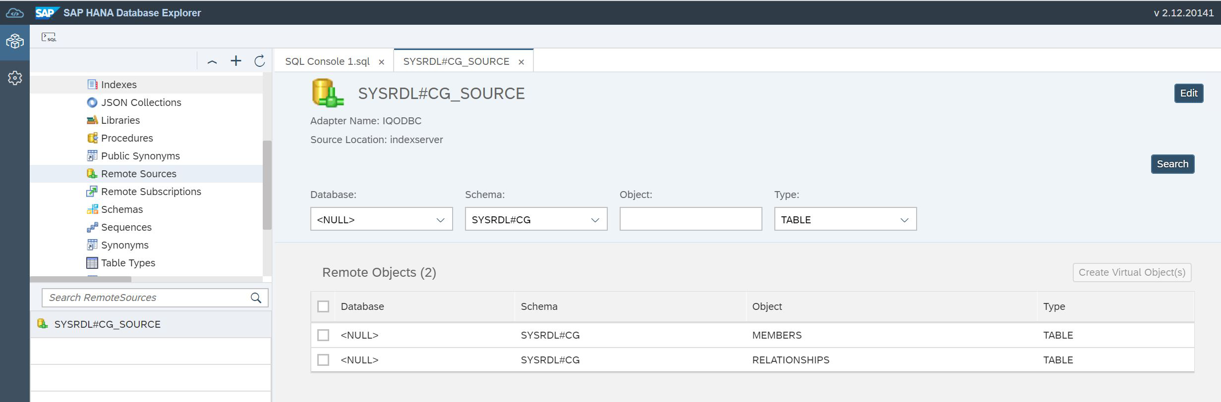
Figure 19
Find both tables, set the checkboxes in front of the tables and click the Create Virtual Object (s) button, as shown in Figure 20.
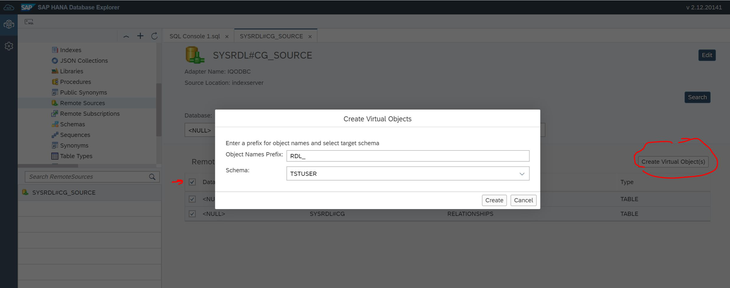
Figure 20
We have the ability to specify the schema in which virtual tables will be created. And there you need to specify a prefix so that these tables are easier to find. After that, we can select Table in the navigator, see our tables and see the data (Fig. 21).

Figure 21
At this step, it is important to pay attention to the filter at the bottom left. Our user name or our TSTUSER scheme should be indicated there.
You are almost done. We created tables in the lake and loaded data into them, and to access them from the HANA level, we have virtual tables. We are ready to create a new object - a graph (Fig. 22).
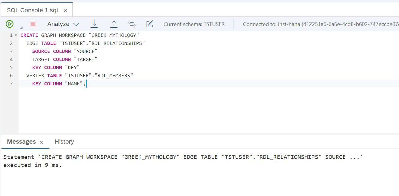
Figure 22
SCRIPT:
CREATE GRAPH WORKSPACE "GREEK_MYTHOLOGY"
  EDGE TABLE "TSTUSER"."RDL_RELATIONSHIPS"
    SOURCE COLUMN "SOURCE"
    TARGET COLUMN "TARGET"
    KEY COLUMN "KEY"
  VERTEX TABLE "TSTUSER"."RDL_MEMBERS"
    KEY COLUMN "NAME";
Everything worked, the count is ready. And you can immediately try to make some simple query to the graph data, for example, find all the daughters of Chaos and all the daughters of these daughters. For this we will be helped by Cypher - a language for graph analysis. It was specially created for working with graphs, convenient, simple and helps to solve complex problems. We just need to remember that the Cypher script needs to be wrapped in a SQL query using a table function. Look how our task is solved in this language (Fig. 23).

Figure 23
SCRIPT:
SELECT * FROM OPENCYPHER_TABLE( GRAPH WORKSPACE "GREEK_MYTHOLOGY" QUERY
    '
	MATCH p = (a)-[*1..2]->(b)
	WHERE a.NAME = ''Chaos'' AND ALL(e IN RELATIONSHIPS(p) WHERE e.TYPE=''hasDaughter'')
	RETURN b.NAME AS Name
	ORDER BY b.NAME
    '
)
Let's check how the visual SAP HANA graph analysis tool works. To do this, select Graph Workspace in the navigator (Fig. 24).
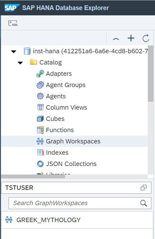
Figure 24
And now you can see our graph (fig. 25).
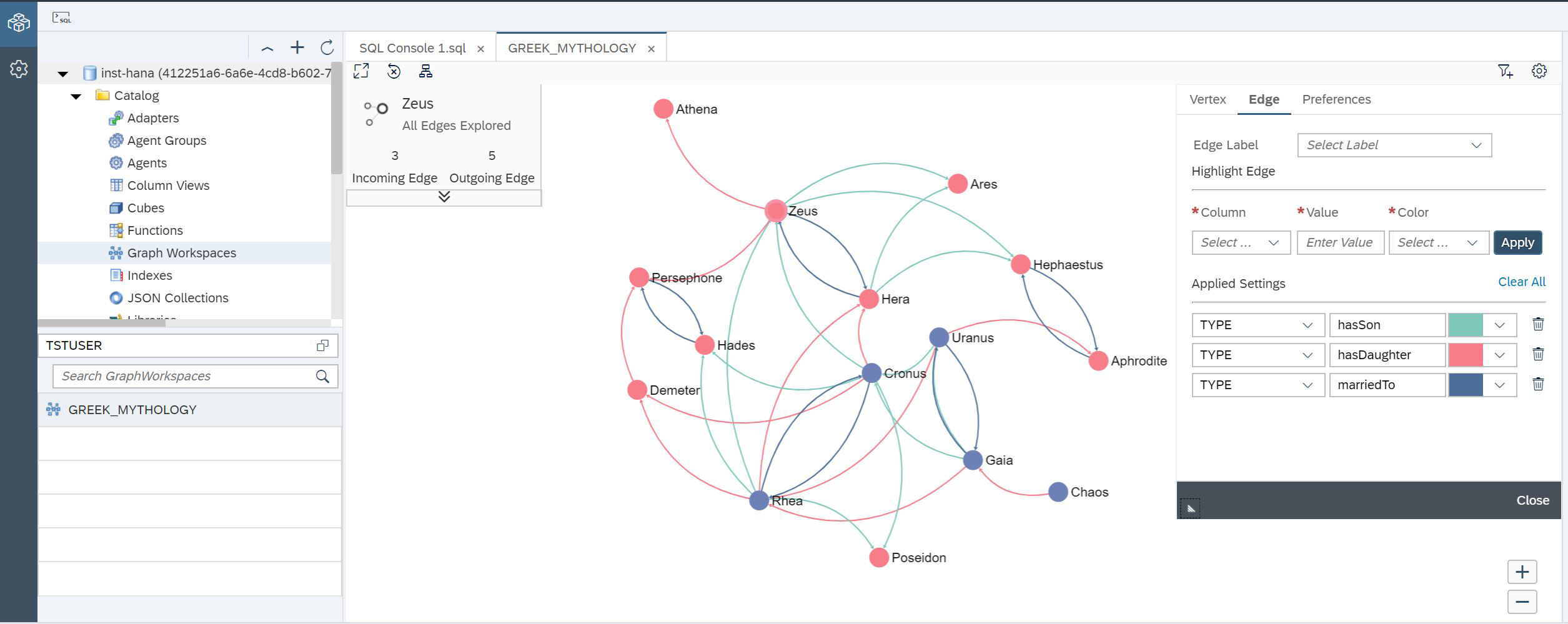
Figure 25
You see a graph that has already been colored. We did this using the settings on the right side of the screen. In the upper left corner, detailed information on the node that is currently selected is shown.
Well ... We did it. The data is in the data lake, and we analyze it with tools in SAP HANA. One technology computes the data, while the other is responsible for storing it. When graph data is processed, it is requested from the data lake and transferred to SAP HANA. Can we speed up our inquiries? How to make data stored in RAM and not loaded from the data lake? There is a simple but not very beautiful way - to create a table in which to load the contents of the data lake table (Fig. 26).

Figure 26
SCRIPT:
CREATE COLUMN TABLE MEMBERS AS (SELECT * FROM "TSTUSER"."RDL_MEMBERS")But there is another way - this is the application of data replication to the RAM of SAP HANA. This can provide better performance for SQL queries than accessing data stored in a data lake using a virtual table. You can switch between virtual and replication tables. To do this, add a replica table to the virtual table. This can be done using the ALTER VIRTUAL TABLE statement. After that, a query using a virtual table automatically accesses the replica table, which is located in the SAP HANA RAM. Let's see how to do this, let's experiment. Let's execute such a request (fig. 27).
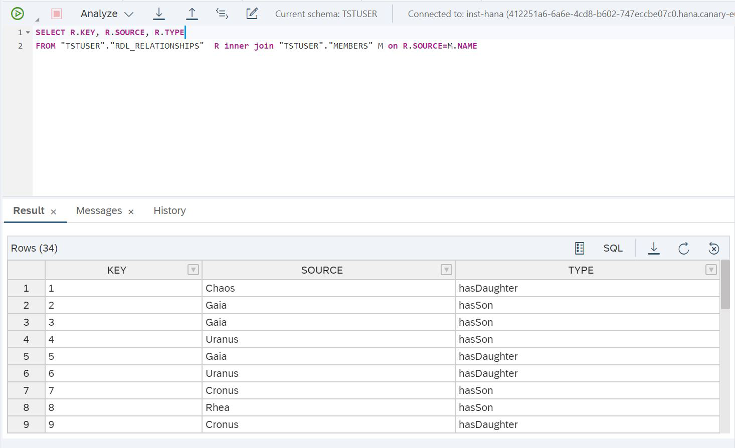
Figure 27
SCRIPT:
SELECT R.KEY, R.SOURCE, R.TYPE
FROM "TSTUSER"."RDL_RELATIONSHIPS"  R inner join "TSTUSER"."MEMBERS" M on R.SOURCE=M.NAME
And let's see how long it took to fulfill this request (Fig. 28).
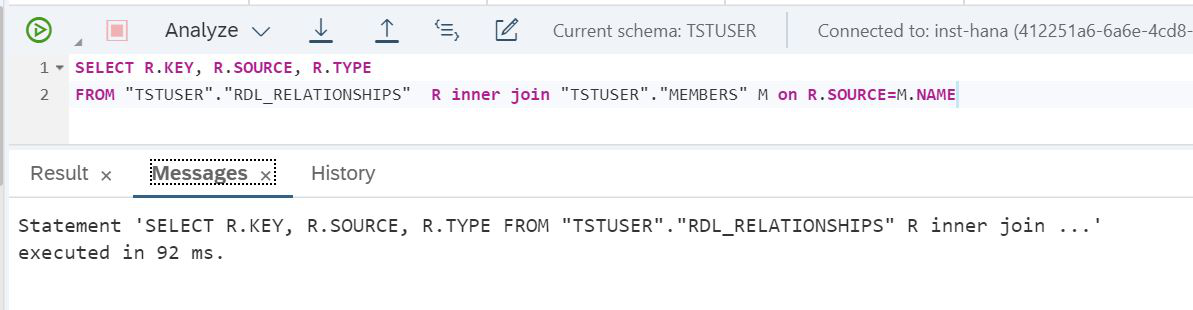
Figure 28
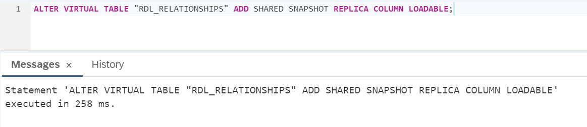
We can see it took 92 milliseconds. Let's enable the replication mechanism. To do this, you need to make ALTER VIRTUAL TABLE of the virtual table, after which the Lake data will be replicated to the SAP HANA RAM.
SCRIPT:
ALTER VIRTUAL TABLE "RDL_RELATIONSHIPS" ADD SHARED SNAPSHOT REPLICA COLUMN LOADABLE;Let's check the execution time as in Figure 29.

Figure 29
We got 7 milliseconds. This is a great result! With minimal effort, we moved the data to RAM. Moreover, if you have finished the analysis and you are satisfied with the performance, you can turn off replication again (Fig. 30).

Figure 30
SCRIPT:
ALTER VIRTUAL TABLE "RDL_RELATIONSHIPS" DROP REPLICA;Now the data is again downloaded from the Lake only upon request, and the SAP HANA RAM is free for new tasks. Today, in my opinion, we did an interesting job and tested SAP HANA Cloud for speed, easy organization of a single data access point. The product will continue to evolve and we expect a direct connection to the data lake in the near future. The new feature will provide a faster download speed of large amounts of information, rejection of unnecessary service data and increase the productivity of operations specific to the data lake. We will create and execute stored procedures directly in the data cloud using SAP IQ technology, that is, we will be able to apply processing and business logic where the data itself is.
Alexander Tarasov, Senior Business Architect, SAP CIS