In the attachment to the article, the path of a particle , cut out materials are provided: path integrals, a double-slit experiment on cold atoms of neon, frames of particle teleportation and other scenes of cruelty and sexual nature.
In my opinion, there can be no other way to consider mathematical formalism to be logically consistent than demonstrating the deviation of its consequences from experience or proving that its predictions do not exhaust the possibilities of observation.
Niels Bohr
In conclusion, the author would like to state that we recognize only two good reasons for rejecting a theory that explains a wide range of phenomena. Firstly, the theory is not internally consistent, and secondly, it is not consistent with experiments.
David Bohm
Earlier we learned where the Schrödinger equation comes from, why it is taken from there, and how it is taken by various methods
Now, we break it into two real equations. To do this, we represent psi in polar form, :
S — , R — . , , , — -, ( ).
, . , S -, - - :
, -, , , , S, , , , . , , . -.
— , . , , , . , , , .
, , , . . . , , , .
, .
, , , . , ( - ). :
()
, , , : ,
, . . .
-, :
using LinearAlgebra, SparseArrays, Plots

const ħ = 1.0546e-34 # J*s
const m = 9.1094e-31 # kg
const q = 1.6022e-19 # Kl
const nm = 1e-9 # m
const fs = 1e-12; # s

function wavefun()

    gauss(x) = exp( -(x-x0)^2 / (2*σ^2) + im*x*k )
    k = m*v/ħ

    #
    Vm = spdiagm(0 => V )
    H = spdiagm(-1 => ones(Nx-1), 0 => -2ones(Nx), 1 => ones(Nx-1) )
    H *= ħ^2 / ( 2m*dx^2 )
    H += Vm

    A = I + 0.5im*dt/ħ * H #
    B = I - 0.5im*dt/ħ * H #
    psi = zeros(Complex, Nx, Nt)
    psi[:,1] = gauss.(x)

    for t = 1:Nt-1

        b = B * psi[:,t]
        #       A*psi = b
        psi[:,t+1] = A \ b
    end

    return psi
end
dx = 0.05nm # x step
dt = 0.01fs # t step
xlast = 400nm
Nt = 260 # Number of time steps
t = range(0, length = Nt, step = dt)
x = [0:dx:xlast;]
Nx = length(x) # Number of spatial steps
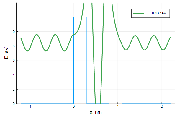
a1 = 200nm
a2 = 200.5nm # 5
a3 = 205nm
a4 = 205.5nm
#V = [ a1<xi<a2 ? 2q : 0.0 for xi in x ] # 2 eV
V = [ a1<xi<a2 || a3<xi<a4 ? 2q : 0.0 for xi in x ] # 2 eV
x0 = 80nm # Initial position
σ = 20nm # gauss width
v = -120nm/fs;
@time Psi = wavefun()
P = abs2.(Psi);
function ψ(xi, j)
k = findfirst(el-> abs(el-xi)<dx, x)
k == nothing && ( k = 1 )
Psi[k, j]
end
function corpusculaz(n)
X = zeros(n, Nt)
X[:,1] = x0 .+ σ*randn(n)
for j in 2:Nt, i in 1:n
U = ħ/(2m*dx) * imag( ( ψ(X[i,j-1]+dx, j) - ψ(X[i,j-1]-dx, j) ) / ψ(X[i,j-1], j) )
X[i,j] = X[i,j-1] - U*dt
end
X
end
@time X = corpusculaz(20);
plot(x, P[:, 1], legend = false)
plot!(x, P[:, 80], legend = false)
scatter!( X[:,1], zeros(20) )
scatter!( X[:,80], zeros(20) )
. — , . :
, . , , !
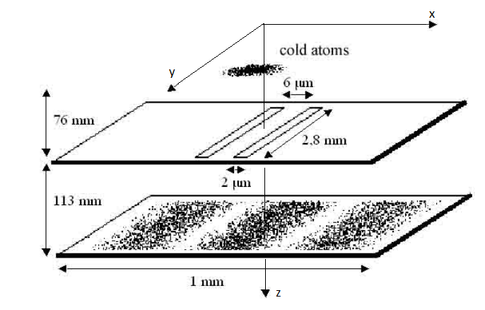
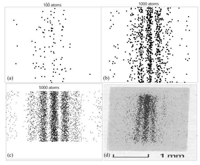
, . Double-slit interference with ultracold metastable neon atoms — - .
using Random, Gnuplot, Statistics
#
function trapez(f, a, b, n)
    h = (b - a)/n
    result = 0.5*(f(a) + f(b))
    for i in 1:n-1
        result += f(a + i*h)
    end
    result * h
end
#
function rk4(f, x, y, h)
    k1 = h * f(x       , y        )
    k2 = h * f(x + 0.5h, y + 0.5k1)
    k3 = h * f(x + 0.5h, y + 0.5k2)
    k4 = h * f(x +    h, y +    k3)

    return y + (k1 + 2*(k2 + k3) + k4)/6.0
end
const ħ = 1.055e-34 # J*s
const kB = 1.381e-23 # J*K-1
const g = 9.8 # m/s^2
const l1 = 76e-3 # m
const l2 = 113e-3 # m
const yh = 2.8e-3 # m
const d = 6e-6 # m
const b = 2e-6 # m
const a1 = 0.5(- d - b) #
const a2 = 0.5(- d + b)
const b1 = 0.5( d - b)
const b2 = 0.5( d + b)
const m = 3.349e-26 # kg
const T = 2.5e-3 # K
const σv = sqrt(kB*T/m) #
const σ₀ = 10e-6 # 10 mkm #
const σz = 3e-4 # 0.3 mm # z
const σk = m*σv / (ħ*√3) # 2e8 m/s #
v₀ = zeros(3)
k₀ = zeros(3);: , , -, .
k
, . , , , . , , .
, . , , — . , , , . , , .
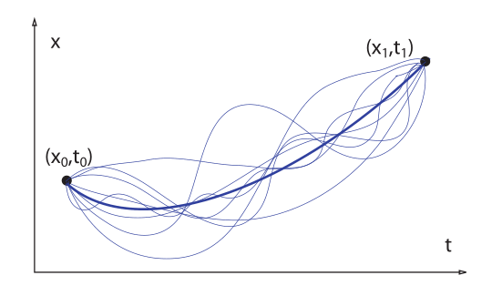
Quantum Mechanics And Path Integrals, A. R. Hibbs, R. P. Feynman, , 3.6 .
,
Z , . ,
, . , X, . :
, :
ε₀(t) = σ₀^2 + ( ħ/(2m*σ₀) * t )^2 + (ħ*t*σv/m)^2
s₀(t) = σ₀ + im*ħ/(2m*σ₀) * t

ρₓ(x, t) = exp( -x^2 / (2ε₀(t)) ) / sqrt( 2π*ε₀(t) )

t₁(v, z) = sqrt( 2*(l1-z)/g + (v/g)^2 ) - v/g
tf1 = t₁(v₀[3], 0) # s #
X1 = range(-100, stop = 100, length = 100)*1e-6
Z1 = range(0, stop = l1, length = 100)
Cron1 = range(0, stop = tf1, length = 100)

P1 = [ ρₓ(x, t) for t in Cron1, x in X1 ]
P1 /= maximum(P1); #

@gp "set title 'Wavefun before the slits'" xlab="Z, mkm" ylab="X, mkm"
@gp :- 1000Z1 1000000X1 P1 "w image notit"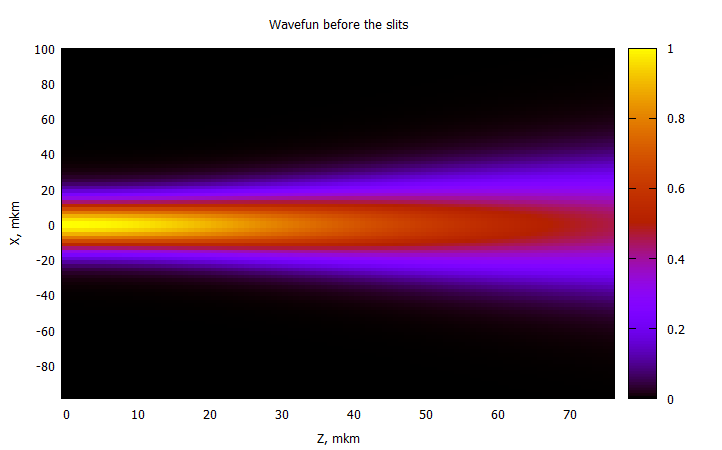
— .
, :
, :
function ρₓ(xᵢ, tᵢ)

    Kₓ(xb, tb, xa, ta) = sqrt( m/(2im*π*ħ*(tb-ta)) ) * exp( im*m*(xb-xa)^2 / (2ħ*(tb-ta)) )

    function subintrho(k)

        ψₓ(x, t) = ( 2π*s₀(t) )^-0.25 * exp( -(x-ħ*k*t/m)^2 / (4σ₀*s₀(t)) + im*k*(x-ħ*k*t/m) )
        subintpsi(x) = Kₓ(xᵢ, tᵢ, x, tf1) * ψₓ(x, tf1)

        ψa = trapez(subintpsi, a1, a2, 200)
        ψb = trapez(subintpsi, b1, b2, 200)

        exp( -k^2 / (2σv^2) ) * abs2(ψa + ψb)
    end

    trapez(subintrho, -10σk, 10σk, 20) / sqrt( 2π*σv^2 )
end
t₂(v, z) = sqrt( 2*(l1+l2-z)/g + (v/g)^2 ) - v/g
tf2 = t₂(v₀[3], 0) # s #
X2 = range(-800, stop = 800, length = 200)*1e-6
Z2 = range(l1, stop = l2, length = 100)
Cron2 = range(tf1, stop = tf2, length = 100)
@time P2 = [ ρₓ(x, t) for t in Cron2, x in X2 ];
P2 /= maximum(P2[4:end,:]);
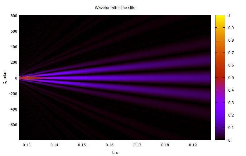
@gp "set title 'Wavefun after the slits'" xlab="t, s" ylab="X, mkm"
@gp :- Cron2[4:end] 1000000X2 P2[4:end,:] "w image notit"2 :
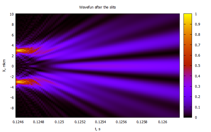
:
. . , ,
, ,
function xbs(t, xo, yo, vo)

    cosϕ = xo / sqrt( xo^2 + yo^2 )
    sinϕ = yo / sqrt( xo^2 + yo^2 )
    atnx = -ħ*t / (2m*σ₀^2)
    sinatnx = atnx / sqrt( atnx^2 + 1)
    cosatnx =    1 / sqrt( atnx^2 + 1)
    cosϕt = cosϕ * cosatnx - sinϕ * sinatnx
    #sinϕt = sinϕ*cosatnx + cosϕ*sinatnx

    σ₀t = sqrt( σ₀^2 + ( ħ*t / (2*m*σ₀) )^2 )

    vo*t + sqrt(xo^2 + yo^2) * σ₀t/σ₀ * cosϕt
end

@gp "set title 'Trajectories before slits'" xlab="t, s" ylab="X, mkm" # "set yrange [-10:10]"

@time for i in 1:80

    x0 = randn()*σ₀
    y0 = randn()*σ₀
    v0 = randn()*σv*1e-4

    prtclᵢ = [ xbs(t,x0,y0,v0) for t in Cron1 ]

    @gp :- Cron1 1000000prtclᵢ "with lines notit lw 2 lc rgb 'black'"
    # slits -4-> -2, 2->4 mkm
end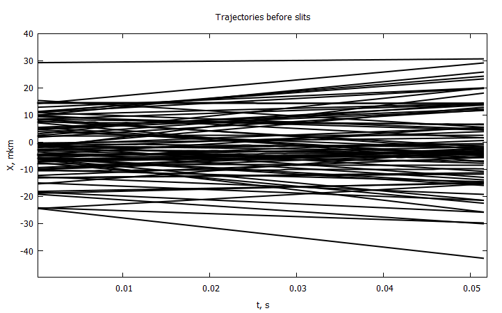
, , , , , . . . , .
Y , , . X . .
" " ,
function Uₓ(t, x)

    γ = -m*x / ( ħ*(t-tf1) )
    β = m/(2ħ) * ( 1/(t-tf1) + 1 / ( tf1*( 1 + (2m*σ₀^2 / (ħ*tf1) )^2 ) ) )
    α = -( 4σ₀^2 * ( 1 + ( ħ*tf1 / (2m*σ₀^2) )^2 ) )^-1

    f(x, u, t) = exp( ( α + im*β )*u^2 + im*γ*u )

    C = f(x, a2, t) - f(x, a1, t) + f(x, b2, t) - f(x, b1, t)
    H = trapez( u-> f(x, u, t) , a1, a2, 400) + trapez( u-> f(x, u, t) , b1, b2, 400)

    return 1/(t-tf1) * ( x - 0.5/(α^2 + β^2) * ( β*imag(C/H) + α*real(C/H) - β*γ ) )
end

init() = bitrand()[1] ? rand()*(b2 - b1) + b1 : rand()*(a2 - a1) + a1
myrng(a, b, N) = collect( range(a, stop = b, length = N ÷ 2) )
n = 1
xx = 0
ξ = 1e-5
while xx < Cron2[end]-Cron2[1]
    n+=1
    xx += (ξ*n)^2
end
n

steps = [ (ξ*i)^2 for i in 1:n1 ]
Cronadapt = accumulate(+, steps, init = Cron2[1] )

function modelsolver(Np = 10, Nt = 100)

    #xo = [ init() for i = 1:Np ] #
    xo = vcat( myrng(a2, a1, Np), myrng(b1, b2, Np) ) #

    xpath = zeros(Nt, Np)
    xpath[1,:] = xo

    for i in 2:Nt, j in 1:Np
        xpath[i,j] = rk4(Uₓ, Cronadapt[i], xpath[i-1,j], steps[i] )
    end

    xpath
end
@time paths = modelsolver(20, n);
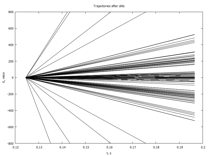
@gp "set title 'Trajectories after the slits'" xlab="t, s" ylab="X, mkm" "set yrange [-800:800]"
for i in 1:size(paths, 2)
@gp :- Cronadapt 1e6paths[:,i] "with lines notit lw 1 lc rgb 'black'"
end- 4 , . 2
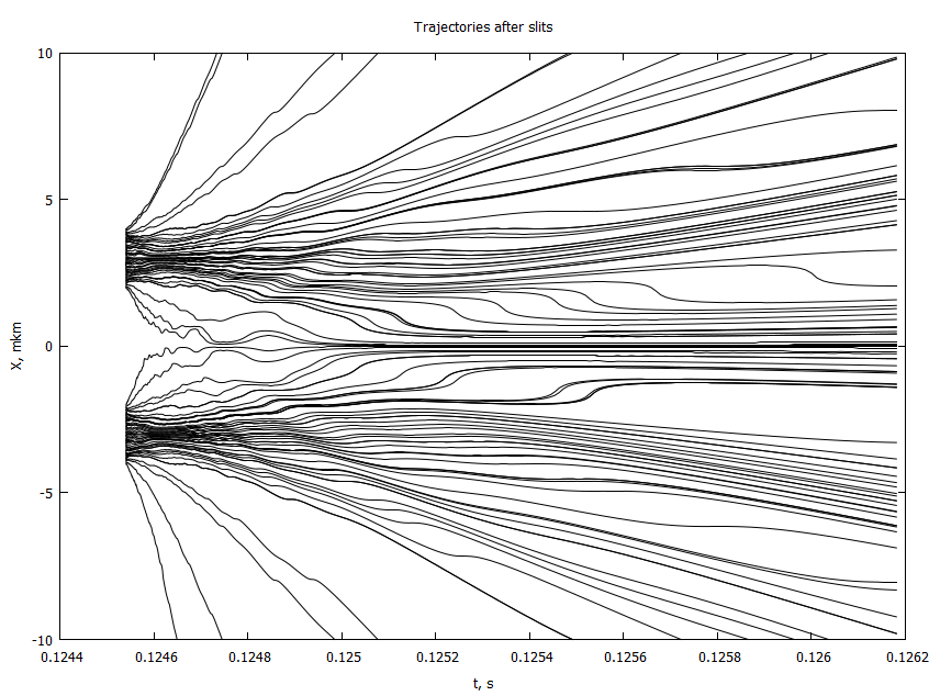
, : , , .
. , ,
function yas(t, xo, yo, vo)

    cosϕ = xo / sqrt( xo^2 + yo^2 )
    sinϕ = yo / sqrt( xo^2 + yo^2 )
    atnx = -ħ*t / (2m*σ₀^2)
    sinatnx = atnx / sqrt( atnx^2 + 1)
    cosatnx =    1 / sqrt( atnx^2 + 1)
    #cosϕt = cosϕ * cosatnx - sinϕ * sinatnx
    sinϕt = sinϕ*cosatnx + cosϕ*sinatnx

    σ₀t = sqrt( σ₀^2 + ( ħ*t / (2*m*σ₀) )^2 )

    vo*t + sqrt(xo^2 + yo^2) * σ₀t/σ₀ * sinϕt
end

function modelsolver2(Np = 10)

    Nt = length(Cronadapt)
    xo = [ init() for i = 1:Np ]
    #xo = vcat( myrng(a2, a1, Np), myrng(b1, b2, Np) )

    xcoord = copy(xo)
    ycoord = zeros(Np)

    for i in 2:Nt, j in 1:Np
        xcoord[j] = rk4(Uₓ, Cronadapt[i], xcoord[j], steps[i] )
    end

    for (i, x) in enumerate(xo)

        y0 = randn()*yh
        v0 = 0 #randn()*σv*1e-4

        ycoord[i] = yas(Cronadapt[end], x, y0, v0)
    end

    xcoord, ycoord
end

@time X, Y = modelsolver2(100);

@gp "set title 'Impacts on the screen'" xlab="X, mm" ylab="Y, mm"# "set xrange [-1:1]"
@gp :- 1000X 1000Y "with points notit pt 7 ps 0.5 lc rgb 'black'"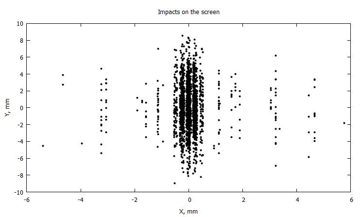
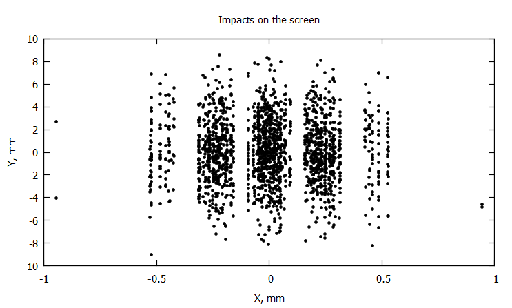
, , . , ,
, , , , , — , .
- Measurement in the de Broglie-Bohm interpretation: Double-slit, Stern-Gerlach and EPR-B —
- — : , - - — ..